1. Introduction & History of Planetary Science

Learning objectives: By the end of this lecture, you will be able to describe the scope of planetary science, explain how the field has evolved from antiquity to the space age, and identify the key properties and classification of solar system bodies.

See also

Slides: Download Lecture 1 (PDF)

Recording: Watch Lecture 1 on YouTube (see Recordings)

1.1. A pale blue dot

On 14 February 1990, the Voyager 1 spacecraft turned its camera back toward the inner solar system one last time. From a distance of 6 billion km, about 40 AU, it captured an image in which Earth appears as a tiny speck, less than a single pixel, suspended in a scattered beam of sunlight (Fig. 1.1). Carl Sagan, who had campaigned for years to have the photograph taken, wrote: “Look again at that dot. That’s here. That’s home. That’s us” [Sagan, 1994]. Minutes later, Voyager’s cameras were switched off for good.

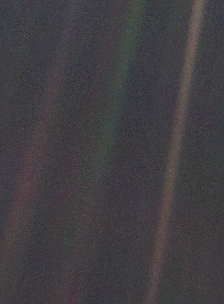
Fig. 1.1 The Pale Blue Dot. Earth appears as a tiny bright speck roughly halfway down the rightmost sunbeam. Captured by Voyager 1 on 14 February 1990 from approximately 6 billion km (40 AU). Image PIA00452. Credit: NASA/JPL-Caltech.

The Pale Blue Dot is one frame in a much larger 60-frame “Family Portrait” mosaic that Voyager 1 returned the same day, the only time a spacecraft has imaged the entire planetary system from outside (Fig. 1.2).

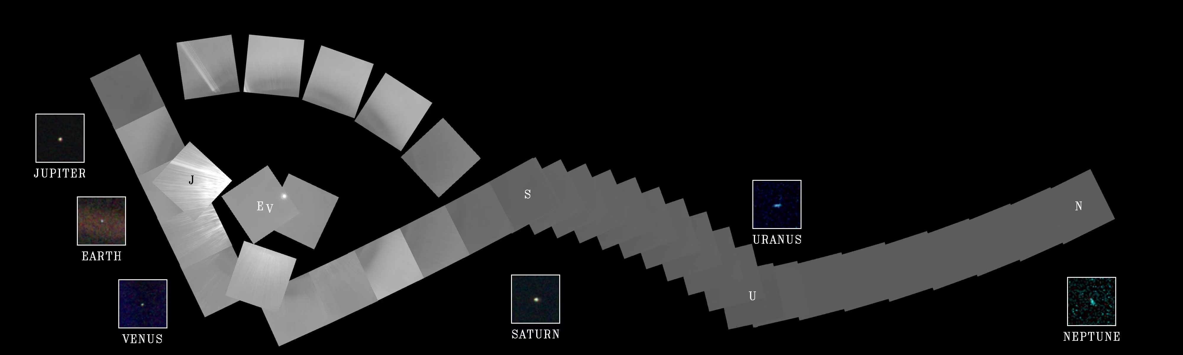
Fig. 1.2 The Voyager 1 “Family Portrait” of the solar system, 14 February 1990, taken from approximately 6 billion km. Six planets are visible across this 60-frame mosaic spanning roughly 70 degrees of sky: Venus, Earth, Jupiter, Saturn, Uranus, and Neptune. Mercury was too close to the Sun to be seen, and Mars showed only a thin sunlit crescent from Voyager 1’s viewpoint and could not be detected; Pluto was too small and distant to image. The Pale Blue Dot (Fig. 1.1) is a zoom into the Earth frame. Credit: NASA/JPL-Caltech, PIA00451.

A second image taken from lunar orbit two decades earlier captured the same essential idea from much closer in: Earth as a finite, fragile world set against an empty sky (Fig. 1.3).

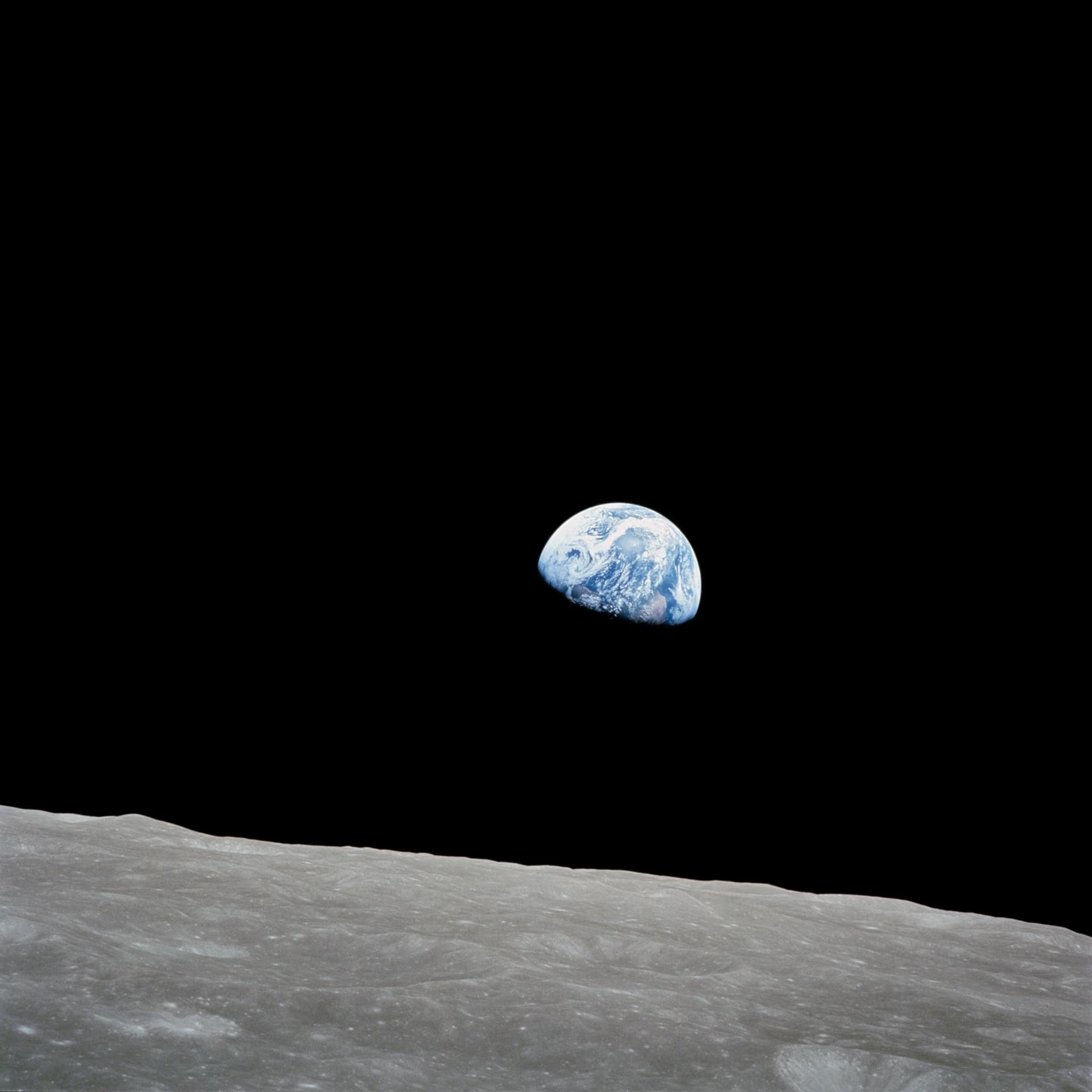
Fig. 1.3 “Earthrise”, Apollo 8, 24 December 1968. Earth rises above the lunar limb during the first crewed mission to leave Earth orbit. The image is widely credited with shifting public perception of Earth as a single, finite system, an early articulation of the comparative-planetology perspective that this course adopts throughout. NASA image AS8-14-2383. Credit: NASA / William Anders.

That image captures something essential about planetary science: it asks us to see our own world not as the centre of the universe, but as one planet among many, a physical system that can be studied, compared, and understood. This course is built around three questions that drive that effort:

1. How did our solar system form, and is it typical? Before 1992, we knew of exactly zero planets outside our solar system. Today we have confirmed more than 6,000 exoplanets in over 4,500 systems [NASA Exoplanet Archive, 2026]. Statistical analyses of the Kepler survey suggest that roughly 0.37 to 0.88 rocky, habitable-zone planets exist per Sun-like star (the range bracketing the conservative and optimistic habitable-zone definitions, see Fig. 1.4) [Bryson et al., 2021], implying hundreds of millions of such worlds in the Milky Way alone. Yet we have detailed knowledge of only one planetary system.

2. What determines whether a planet becomes habitable? Venus, Earth, and Mars all formed from the same protoplanetary disk, likely with similar initial compositions. All three may have had early liquid water. Yet today Venus has a 464 °C surface beneath 92 bar of CO\(_2\), Earth has oceans and a biosphere, and Mars is a cold desert with an atmosphere thinner than 1% of Earth’s. Understanding why they diverged is one of the central puzzles of planetary science.

3. Are we alone? The James Webb Space Telescope (JWST) is currently attempting to detect and characterise atmospheres on rocky exoplanets, including the TRAPPIST-1 system. Within your careers, this question may become answerable, but only if we understand what makes a planet habitable in the first place.

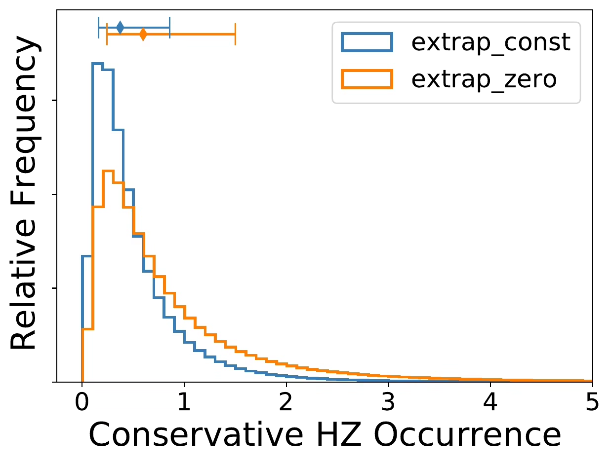
Fig. 1.4 Posterior probability density on \(\eta_\oplus\), the average number of rocky habitable-zone planets per Sun-like star, derived from Kepler data, for the conservative habitable-zone definition (moist-greenhouse inner edge to maximum-greenhouse outer edge, the range over which liquid water can be reliably maintained at the surface). The two coloured posteriors bracket the unknown survey completeness at orbital periods beyond Kepler’s 500-day calibration limit: the blue curve (legend extrap_const) assumes that the detection completeness stays constant at its 500-day value, which overestimates completeness for longer periods and therefore gives a lower bound on \(\eta_\oplus\); the orange curve (legend extrap_zero) assumes that completeness drops to zero beyond 500 days, underestimating completeness and therefore giving an upper bound on \(\eta_\oplus\). The headline central values from Bryson et al. [2021] are \(\eta_\oplus \approx 0.37\) (extrap_const) and \(\eta_\oplus \approx 0.60\) (extrap_zero); the wider optimistic habitable-zone definition (inner edge at the recent-Venus insolation bound, outer edge at early-Mars) raises these to \(\approx 0.58\) and \(\approx 0.88\). The numbers are the diamond markers above the histograms (medians of the posterior, with 68% credible intervals), not the histogram modes. Either way, habitable-zone rocky planets around Sun-like stars are common.

Every topic in this course, from orbital dynamics and interior structure to atmospheric physics and surface geology, connects back to these three questions. By the end, you will have the tools to think about them quantitatively.

1.2. What is a planet?

The word “planet” derives from the Greek planetes (πλανήτης), meaning “wanderer.” To ancient observers, the planets were the five visible points of light (Mercury, Venus, Mars, Jupiter, and Saturn) that moved against the fixed background of stars. Together with the Sun and Moon, these seven wanderers gave us the seven days of the week.

For over two millennia, the list of planets seemed settled. That changed with the invention of the telescope. William Herschel discovered Uranus in 1781, the first planet found in modern times. In 1846, Johann Galle observed Neptune at a position predicted independently by Urbain Le Verrier and John Couch Adams from perturbations in Uranus’s orbit, a triumph of Newtonian mechanics. And in 1930, Clyde Tombaugh discovered Pluto at Lowell Observatory after a painstaking photographic search.

But Pluto was always an oddity: small, icy, with an eccentric and inclined orbit that crosses Neptune’s. When astronomers began discovering other large objects beyond Neptune in the 1990s and 2000s, culminating in the discovery of Eris in 2005 by Brown et al. [2005], which appeared comparable in size to Pluto, the question became unavoidable: either these new objects were also planets, or Pluto was not. The 2015 New Horizons flyby (Fig. 1.5) revealed an unexpectedly active world, complicating the debate further.

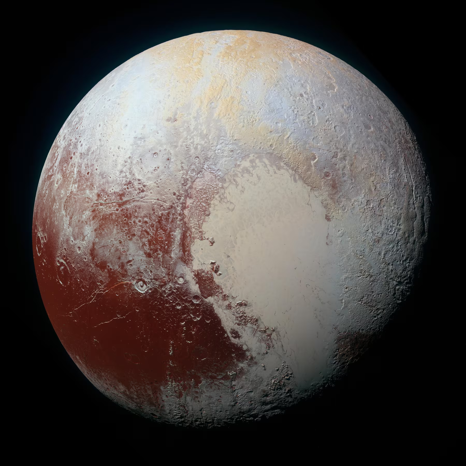
Fig. 1.5 Pluto in enhanced colour from NASA’s New Horizons spacecraft, July 2015. The dark reddish region on the left (Cthulhu Macula) and the bright nitrogen-ice plains visible to the right (the western edge of Tombaugh Regio, the “heart”) highlight a surface diversity that was completely unexpected for a body of Pluto’s size. New Horizons revealed water-ice mountains, glacial flows, and possible cryovolcanism, reigniting debate over Pluto’s planetary status. Credit: NASA/JHUAPL/SwRI.

1.2.1. The IAU definition

On 24 August 2006, the International Astronomical Union (IAU) adopted Resolution 5A, establishing three criteria for a body in the solar system to be classified as a planet [International Astronomical Union, 2006]:

1. It is in orbit around the Sun.

2. It has sufficient mass for its self-gravity to overcome rigid body forces, so that it assumes a hydrostatic equilibrium (nearly round) shape.

3. It has cleared the neighbourhood around its orbit.

A body satisfying criteria 1 and 2 but not 3 is a dwarf planet. Under this definition, the solar system has eight planets and five officially recognised dwarf planets: Ceres, Pluto, Eris, Makemake, and Haumea. Many additional candidates exist in the Kuiper Belt.

The definition remains debated: “clearing the neighbourhood” is not precisely defined and depends on heliocentric distance, and Earth would not clear its zone if placed at Neptune’s orbit. An alternative geophysical definition proposes that any body massive enough to achieve hydrostatic equilibrium should count as a planet, regardless of its orbital dynamics [Runyon et al., 2017]. Under this broader definition, the solar system would have well over 100 planets.

For this course, the exact classification matters less than the physics. The important point is that the solar system contains a continuous spectrum of objects, from dust grains to gas giants, governed by the same physical laws.

1.3. Brief history of planetary science

Planetary science as a discipline is remarkably young, but its roots reach back to the earliest recorded observations.

1.3.1. Ancient and pre-telescopic astronomy

Babylonian astronomers systematically tracked planetary positions as early as 1800 BCE, developing arithmetical methods to predict conjunctions and oppositions. Greek natural philosophers constructed geometric models: Aristotle’s geocentric spheres (~350 BCE) and Ptolemy’s epicyclic system (~150 CE) remained the standard framework for over a millennium.

The Copernican revolution began in 1543, when Nicolaus Copernicus published De revolutionibus, placing the Sun at the centre (Fig. 1.6). Johannes Kepler refined this model into his three empirical laws of planetary motion (1609 to 1619), replacing circles with ellipses. Isaac Newton’s Principia (1687) showed that all three of Kepler’s laws follow from a single universal law of gravitation, the first grand unification in physics.

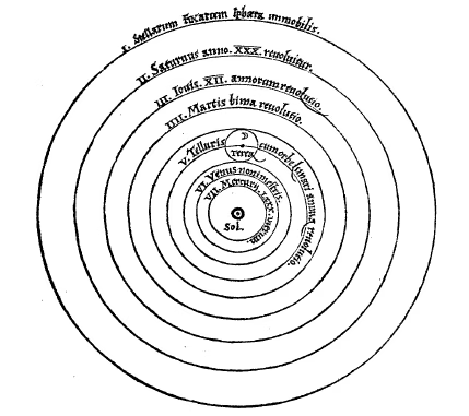
Fig. 1.6 Heliocentric model of the solar system from Copernicus’s De revolutionibus orbium coelestium (1543). The Sun sits at the centre, with the planets orbiting outward in concentric spheres. The Latin inscriptions, from the centre out, read Sol (Sun), Mercurius (Mercury), Venus, Terra (Earth, with the Moon as a small orbit attached), Mars, Iupiter (Jupiter), Saturnus (Saturn), and the outer band Stellarum Fixarum Sphaera Immobilis (the immobile sphere of the fixed stars). This woodcut marks the conceptual shift from the geocentric cosmology that had dominated for over a millennium. Credit: Nicolaus Copernicus, public domain.

1.3.2. The telescopic era

Galileo Galilei’s telescope observations in 1610 transformed planetary science from mathematics into a physical science. He discovered four moons orbiting Jupiter (now called the Galilean moons; see Fig. 1.7), observed the phases of Venus (confirming it orbits the Sun), and resolved Saturn’s rings (though he could not interpret their structure).

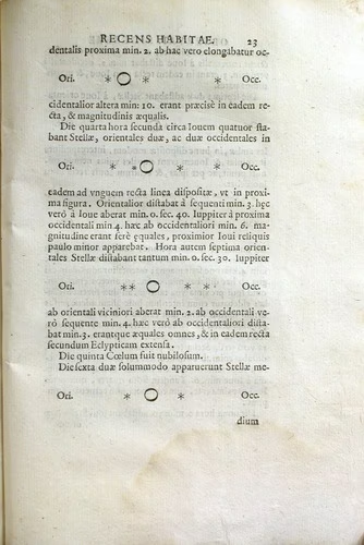
Fig. 1.7 Page from Galileo’s Sidereus Nuncius (1610) showing his observations of Jupiter and its four largest moons, named here the Medicea Sidera (Medicean Stars) in honour of Galileo’s Medici patrons. Each row records the positions of the moons (small dots) relative to Jupiter (open circle) on successive nights. The systematic motion of the four points, repeating with periods of days, was direct evidence that not all celestial bodies orbit the Earth. Simon Marius proposed the mythological names Io, Europa, Ganymede, and Callisto in 1614; these gradually replaced the Medicean designation and are the names you will meet in Lecture 11. Credit: Galileo Galilei, public domain.

Over the following centuries, improving telescopes revealed surface features on Mars, the Great Red Spot on Jupiter, and the detailed ring structure of Saturn.

The 19th century brought spectroscopy, allowing astronomers to determine atmospheric compositions remotely for the first time. Photography enabled systematic surveys, and the discoveries of Uranus, Neptune, and Pluto progressively expanded the known solar system.

1.3.3. The space age

The modern era of planetary science began on 14 December 1962, when NASA’s Mariner 2 flew past Venus, the first spacecraft to successfully visit another planet. This flyby revealed Venus’s extreme surface temperature, overturning earlier speculation about habitable conditions beneath its clouds.

The pace of exploration accelerated rapidly. Mariner 4 returned the first close-up images of Mars in 1965 (Fig. 1.8), revealing a cratered, apparently dead world, not the canal-laced surface some had imagined. The Soviet Venera 7 achieved the first landing on another planet (Venus, 1970). NASA’s Viking landers (1976) conducted the first experiments searching for life on Mars. The twin Voyager spacecraft (launched 1977) exploited a rare planetary alignment to conduct a grand tour of the outer solar system, visiting Jupiter, Saturn, Uranus, and Neptune between 1979 and 1989 (Fig. 1.9).

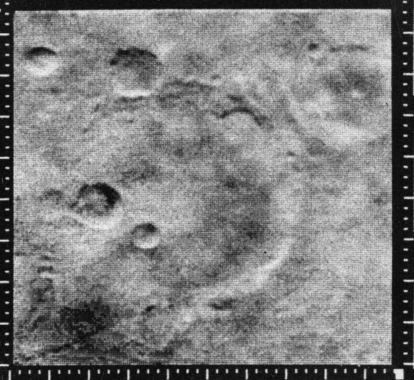
Fig. 1.8 The first close-up image of another planet’s surface: Mariner 4, 15 July 1965. Mariner 4 returned 21 frames during the brief Mars encounter, of which this is one of the most reproduced. The heavily cratered, Moon-like terrain visible here decisively ended speculation about Martian canals and surface vegetation. Mars’s geology and atmosphere are revisited in Lecture 10. Credit: NASA/JPL.

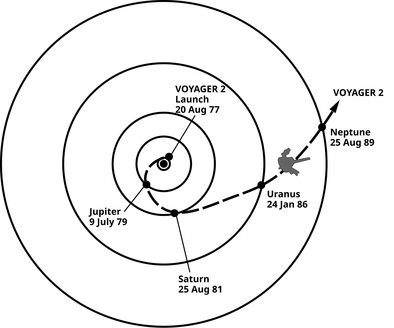
Fig. 1.9 Trajectory of NASA’s Voyager 2 spacecraft during its grand tour of the outer solar system, with the spacecraft itself shown schematically as the small grey silhouette near the Uranus-Neptune segment of the trajectory. Gravity assists at Jupiter (1979), Saturn (1981), Uranus (1986), and Neptune (1989) successively redirected the spacecraft to each subsequent target, a trajectory made possible by a rare alignment of the outer planets that occurs roughly once every 175 years. Voyager 1, launched two weeks later on a faster trajectory, flew only by Jupiter (1979) and Saturn (1980) before being deflected northward out of the ecliptic. Both spacecraft are now in interstellar space: Voyager 1 crossed the heliopause in 2012, Voyager 2 in 2018. Credit: NASA/JPL, public domain.

1.3.4. The exoplanet revolution

In 1992, Aleksander Wolszczan and Dale Frail announced the discovery of planets orbiting a pulsar, the first confirmed exoplanets [Wolszczan and Frail, 1992]. Three years later, Michel Mayor and Didier Queloz detected 51 Pegasi b, the first planet orbiting a Sun-like star: a “hot Jupiter” with a 4.2-day orbit that challenged all existing formation theories [Mayor and Queloz, 1995]. The French-led CoRoT space mission (Convection, Rotation and planetary Transits) then announced the first transiting rocky exoplanet, CoRoT-7b, in 2009, a super-Earth with a measured radius of \(1.58\,\Rearth\) and a 0.85-day orbit [Léger et al., 2009]. NASA’s Kepler mission [Borucki et al., 2010] operated from 2009 to 2018 and discovered thousands of transiting exoplanets, while the ongoing TESS mission (Transiting Exoplanet Survey Satellite, launched 2018) surveys the brightest nearby stars. JWST, launched in December 2021, is now characterising exoplanet atmospheres through transmission and emission spectroscopy (Lecture 13). The cumulative tally of confirmed detections is shown in Fig. 1.10.

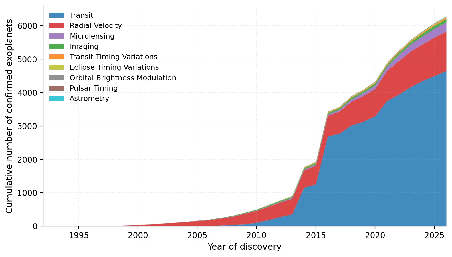
Fig. 1.10 Cumulative number of confirmed exoplanets per discovery year, colour-coded by detection method. The first detection (1992, pulsar timing) was followed by the radial-velocity revolution of the late 1990s and 2000s, and then the explosion of transit discoveries during and after NASA’s Kepler mission (2009 to 2018). The visible step-jumps in 2014 and 2016 are the Kepler team’s statistical-validation batch releases, in which hundreds (2014) and over a thousand (2016) Kepler candidates were promoted to confirmed planets simultaneously rather than one-by-one. Credit: NASA Exoplanet Archive (Caltech), accessed 2026-05-08 [NASA Exoplanet Archive, 2026]. Course-original figure.

The same set of detections plotted in mass-period space (Fig. 1.11) reveals strong selection biases: large short-period planets dominate the upper-left of the diagram, while Earth analogues in the lower-right remain sparsely populated.

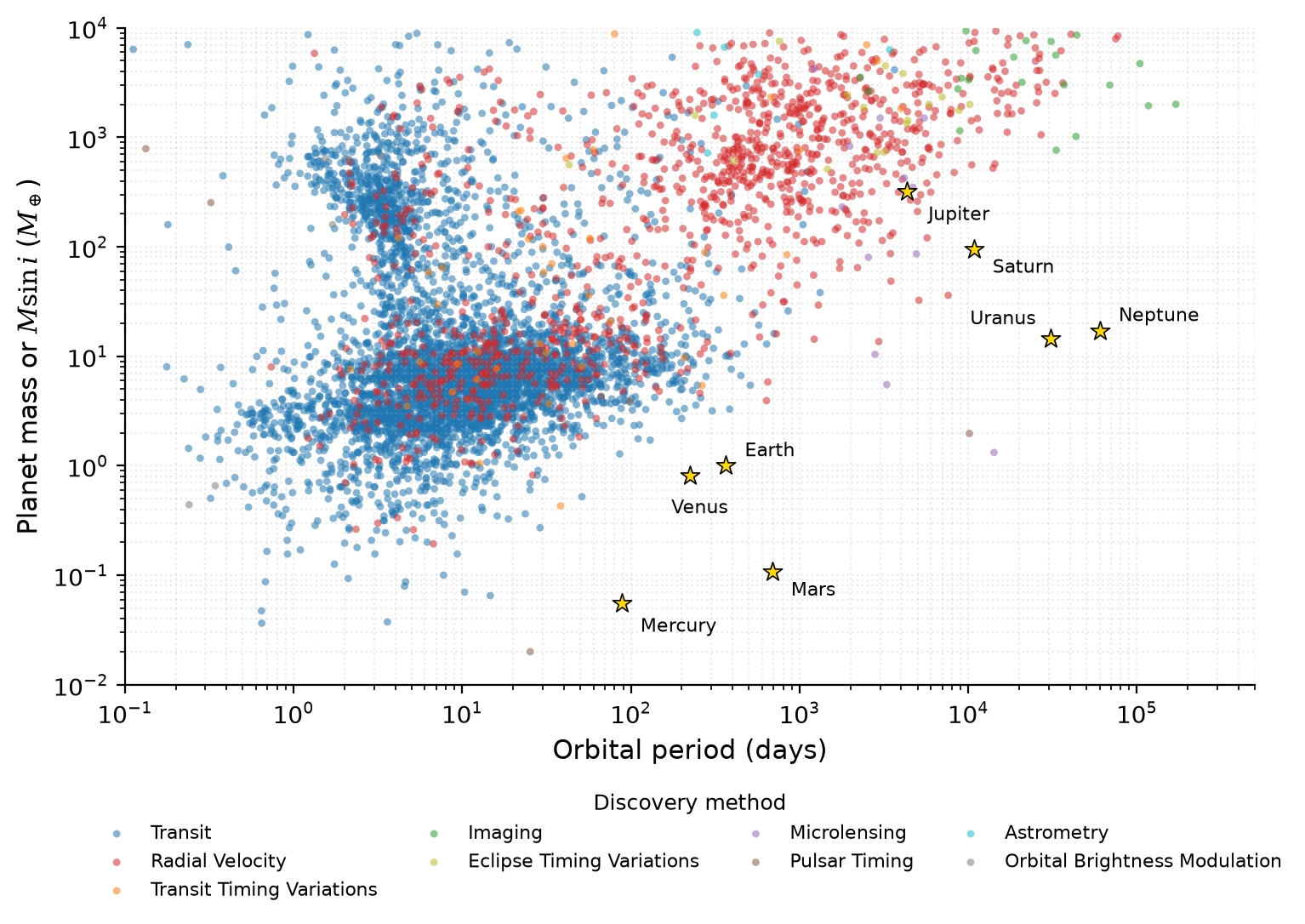
Fig. 1.11 Planet mass (or \(M\sin i\)) versus orbital period for all confirmed exoplanets, colour-coded by detection method, with the eight solar-system planets shown as gold stars for reference. Selection effects favour large, short-period planets in the upper-left of the diagram. The Earth-analogue regime, near mass \(\sim 1\,\Mearth\) and orbital period \(\sim 1\) year, sits in the lower-middle of the plot and remains sparsely populated because radial-velocity and transit surveys with multi-year baselines have only recently begun to access it; future direct-imaging missions (in particular the Habitable Worlds Observatory and the LIFE interferometer concept) are explicitly designed to fill this region by spatially separating reflected or thermal planet light from the host star. Credit: NASA Exoplanet Archive (Caltech), accessed 2026-08-21 [NASA Exoplanet Archive, 2026]. Course-original figure.

Within the small-planet regime, the Kepler sample reveals a bimodal radius distribution (Fig. 1.12) with peaks near \(1.3\,\Rearth\) and \(2.4\,\Rearth\) separated by a “radius valley”, interpreted as the boundary between rocky planets and those retaining a thin H/He envelope.

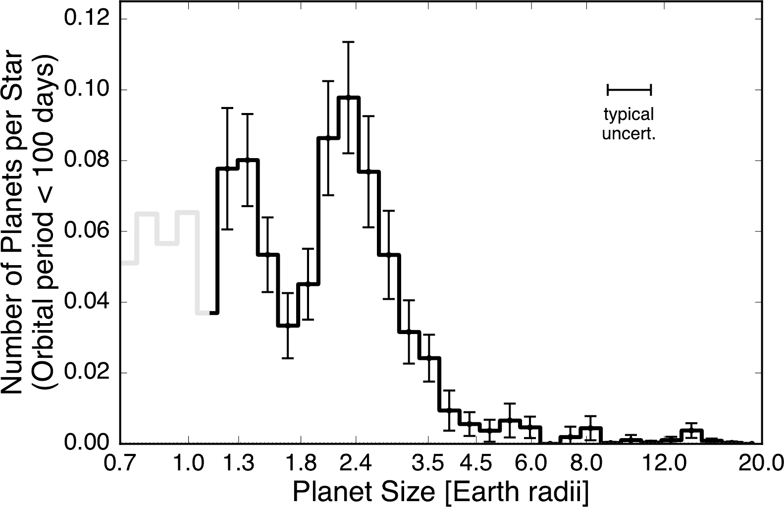
Fig. 1.12 Completeness-corrected histogram of planet radii from the California-Kepler Survey, restricted to planets with orbital periods \(< 100\) d around FGK host stars. The bimodal distribution shows two peaks near \(1.3\,\Rearth\) (super-Earths) and \(2.4\,\Rearth\) (sub-Neptunes) separated by a “radius valley” near \(1.8\,\Rearth\), interpreted as the boundary between rocky planets and those that retain a thin H/He envelope. Error bars are 1-\(\sigma\) from Poisson statistics on the binned detection counts; the light-grey segment below about \(1.1\,\Rearth\) marks the radius range where the Kepler survey suffers from low completeness and the inferred occurrence is unreliable. The “typical uncert.” marker in the upper right is the median radius measurement uncertainty for an individual planet. The radius valley and its implications for atmospheric escape are revisited in Lecture 13. Reproduced from Fulton et al. [2017], Fig. 7 (top panel).

Beyond the demographics, imaging of the young star HL Tauri with the Atacama Large Millimeter/submillimeter Array (ALMA) (Fig. 1.13) provides direct visual evidence of planet formation in progress: concentric gaps in the protoplanetary disk are widely interpreted as carved by forming protoplanets.

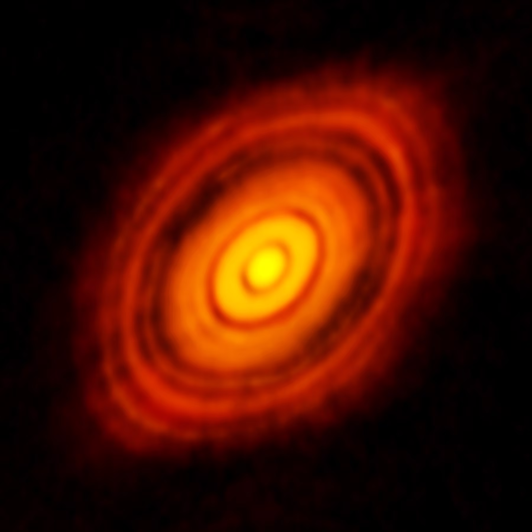
Fig. 1.13 ALMA 1.3 mm continuum image of the protoplanetary disk around the young star HL Tauri (distance \(\sim 140\) pc). The concentric dark gaps are widely interpreted as carved by forming protoplanets, although alternative explanations involving local pile-ups of dust grains at ice lines and other disk substructures remain on the table. ALMA’s \(\sim 5\) AU angular resolution at HL Tau’s distance is what made this multi-ringed substructure visible for the first time. Protoplanetary disks and planet formation are covered in Lecture 2. Credit: ALMA (ESO/NAOJ/NRAO); ALMA Partnership et al. [2015].

The most recent step in exoplanet science has been the direct chemical characterisation of atmospheres. JWST measures the absorption spectrum of starlight that filters through a transiting planet’s atmosphere and identifies individual molecules in it. JWST observed the hot Saturn WASP-39 b in July 2022, and in August 2022 the team of its Near-Infrared Spectrograph (NIRSpec) announced the first unambiguous detection of carbon dioxide in an exoplanet atmosphere (Fig. 1.14) [Rustamkulov et al., 2023]. The 4.3 \(\mu\)m \(\mathrm{CO_2}\) absorption feature is unmistakable; it was the prototype result for the wider JWST exoplanet-atmosphere programme that is now examining dozens of planets and is the principal subject of Lecture 13.

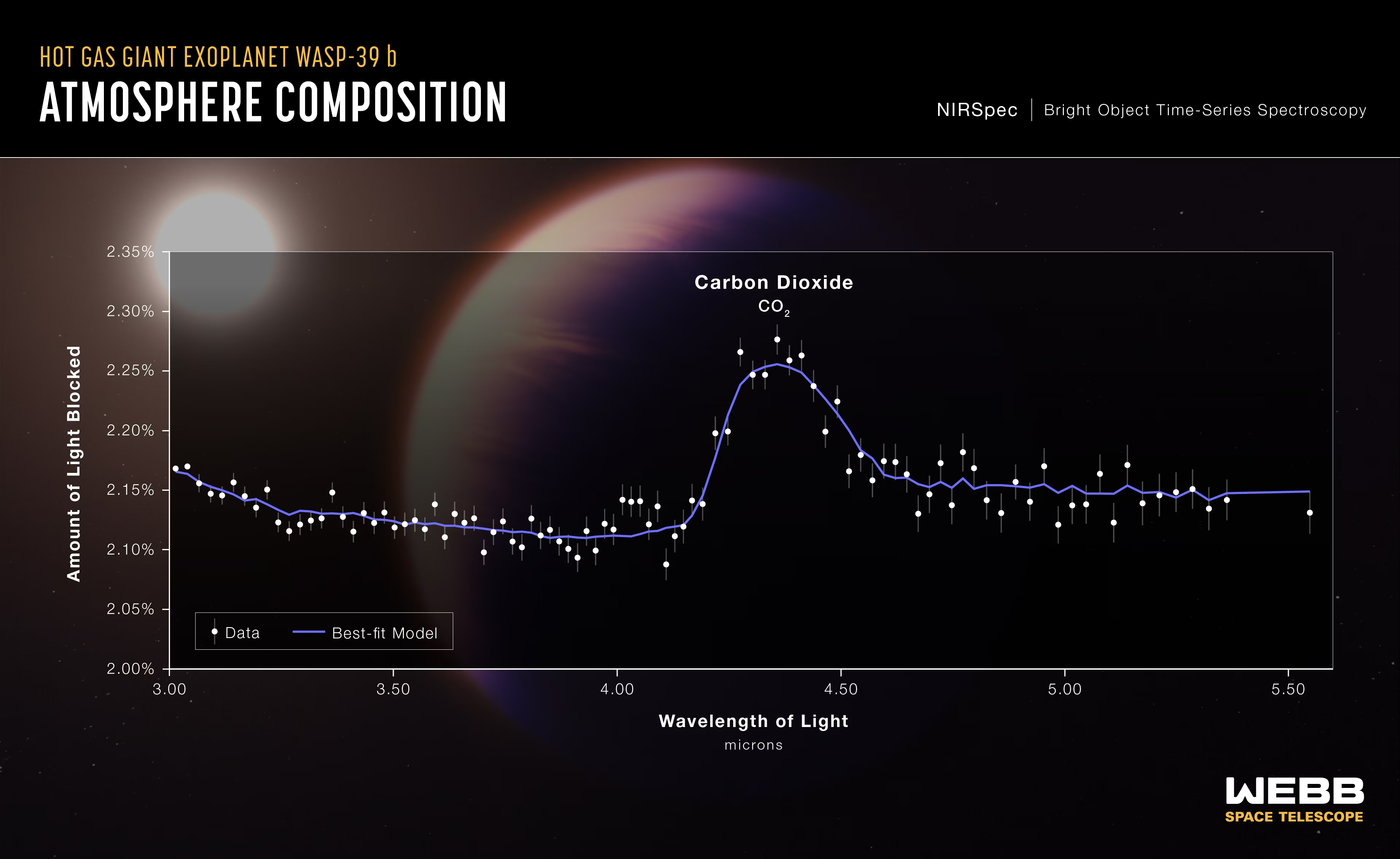
Fig. 1.14 NASA outreach graphic of the first unambiguous detection of carbon dioxide in an exoplanet atmosphere, from JWST/NIRSpec observations of the hot Saturn WASP-39 b (\(0.28\,\Mjup\), comparable in mass to Saturn) in July 2022. The “amount of light blocked” (transit depth) is plotted as a function of wavelength from 3.0 to 5.5 \(\mu\)m. The prominent peak near 4.3 \(\mu\)m is the \(\mathrm{CO_2}\) absorption band. White points are data with uncertainty bars; the blue curve is the best-fit atmospheric model [Rustamkulov et al., 2023]. Image credit: NASA, ESA, CSA, Joseph Olmsted (STScI).

Today, planetary science integrates astronomy, physics, chemistry, geology, and atmospheric science. It spans scales from dust grains in protoplanetary disks to the demographics of planetary systems across the Galaxy.

1.4. Overview of the solar system

1.4.1. Architecture and scale

The solar system extends from the Sun (radius \(\Rsun = 6.96 \times 10^8\) m) to the Oort Cloud, a hypothetical reservoir of comets at roughly \(10^4\) to \(10^5\) AU. Its principal components, from the inside out, are:

• The inner solar system: Four rocky (terrestrial) planets (Mercury, Venus, Earth, Mars) with semi-major axes between 0.39 and 1.52 AU. These are small, dense, and composed primarily of rock and metal.

• The asteroid belt: A population of rocky and metallic bodies between roughly 2.1 and 3.3 AU, dominated by the dwarf planet Ceres (diameter ~940 km). The total mass of the asteroid belt is only ~\(4 \times 10^{-4}\) \(\Mearth\).

• The outer solar system: Four giant planets, Jupiter and Saturn (gas giants) and Uranus and Neptune (ice giants), between 5.2 and 30.1 AU. These are massive, with thick hydrogen-helium envelopes and extensive moon systems.

• The Kuiper Belt and scattered disk: A region of icy bodies beyond Neptune. The classical Kuiper Belt sits at roughly 30 to 50 AU and contains the dwarf planets Pluto, Makemake, and Haumea. The scattered disk extends to much greater distances on more eccentric orbits and contains Eris (Brown et al. [2005]); the inner Oort cloud / detached-object population (Sedna and others) lies further out still.

• The Oort Cloud: A spherical shell of icy bodies at \(10^4\) to \(10^5\) AU, believed to be the source of long-period comets. Its existence is inferred from cometary orbits but has not been directly observed.

The principal solar-system bodies span more than two orders of magnitude in size, from Jupiter (diameter \(\sim 143{,}000\) km, roughly \(29\times\) that of Mercury) down to the largest Kuiper Belt and scattered-disk objects (diameters \(\sim 2{,}000\) to \(2{,}400\) km). Fig. 1.15 brings the four populations introduced above together at true relative size.

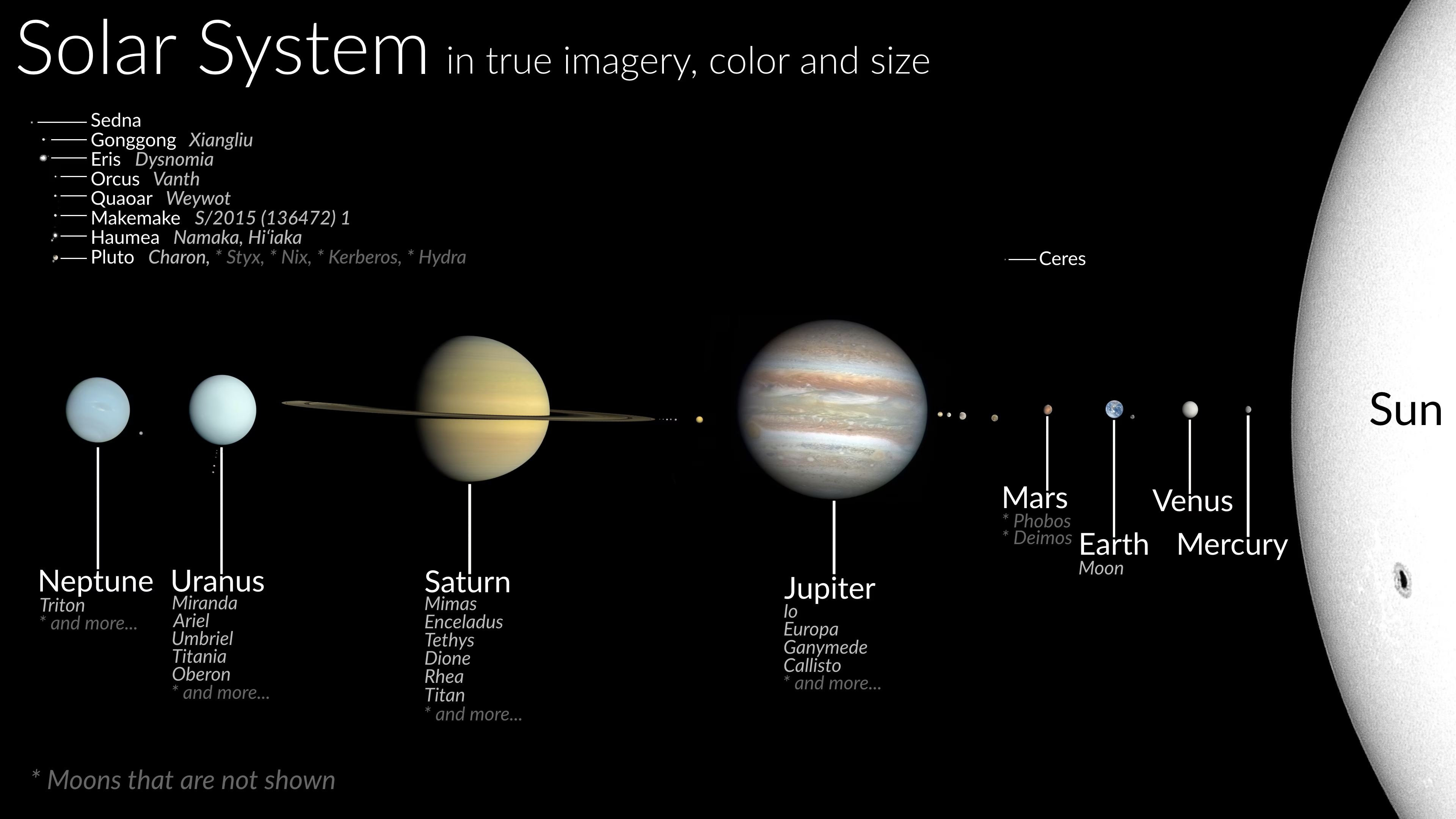
Fig. 1.15 Composite at true relative size of the principal bodies of the solar system, mapping onto the four populations introduced in the text. Inner solar system: Mercury, Venus, Earth (with the Moon), and Mars (with Phobos and Deimos). Asteroid belt: represented by the dwarf planet Ceres. Outer solar system: Jupiter, Saturn, Uranus, and Neptune, each shown with their largest moons (Io, Europa, Ganymede, Callisto for Jupiter; Mimas, Enceladus, Tethys, Dione, Rhea, Titan for Saturn; Miranda, Ariel, Umbriel, Titania, Oberon for Uranus; Triton for Neptune). Kuiper Belt, scattered disk, and detached objects: Pluto (with the labelled moons Charon, Styx, Nix, Kerberos, and Hydra), Haumea (with Namaka and Hi’iaka), Makemake, Quaoar (with Weywot), Orcus (with Vanth), Eris (with Dysnomia), Gonggong (with Xiangliu), and Sedna. The Sun’s limb is shown at right for scale. Body sizes are to scale relative to each other; distances between bodies are not to scale. The Oort Cloud is not depicted since its constituent comet nuclei are individually too small to image. Composite by CactiStaccingCrane (Wikimedia Commons, CC BY-SA 4.0); source imagery: NASA, ESA, ISRO.

1.4.2. Planetary properties

The table below summarises the key physical and orbital properties of the eight planets. Note the enormous dynamic range: Jupiter is over 5,700 times more massive than Mercury, yet both orbit the same star.

Key properties of the eight solar system planets. Data from [NASA Jet Propulsion Laboratory, 2026]. Radii are equatorial; the densities are bulk values based on the volumetric mean radius, so for the oblate giant planets \(\rho\) computed from the tabulated \(M\) and \(R\) comes out up to \(10\%\) low.

Planet	Mass (\(\Mearth\))	Radius (\(\Rearth\))	\(a\) (AU)	\(P\) (yr)	\(e\)	\(\rho\) (kg m\(^{-3}\))
Mercury	0.055	0.383	0.387	0.241	0.206	5427
Venus	0.815	0.949	0.723	0.615	0.007	5243
Earth	1.000	1.000	1.000	1.000	0.017	5514
Mars	0.107	0.532	1.524	1.881	0.093	3934
Jupiter	317.8	11.21	5.203	11.86	0.049	1326
Saturn	95.16	9.45	9.537	29.46	0.054	687
Uranus	14.54	4.01	19.19	84.01	0.047	1271
Neptune	17.15	3.88	30.07	164.8	0.009	1638

Two patterns stand out immediately. First, density decreases with distance (Fig. 1.16): the inner planets have \(\rho > 3900\) kg m\(^{-3}\) (rock and metal), while the outer planets have \(\rho < 1700\) kg m\(^{-3}\) (gas and ice). Saturn is famously less dense than water. The canonical interpretation is that this gradient reflects the temperature structure of the protoplanetary disk: rock condenses everywhere, ices only beyond the snow line at \(\sim 3\) to \(5\) AU, and hydrogen and helium are accreted as gas by the cores that form quickly enough to capture it before the disk dispersed. This picture is the starting point developed in Lecture 2; we will see there that modern formation models continue to refine, and in some places challenge, several parts of it. Second, mass is concentrated in Jupiter (Fig. 1.17): it contains more than twice the mass of all other planets combined. We will quantify this in the blackboard derivation below.

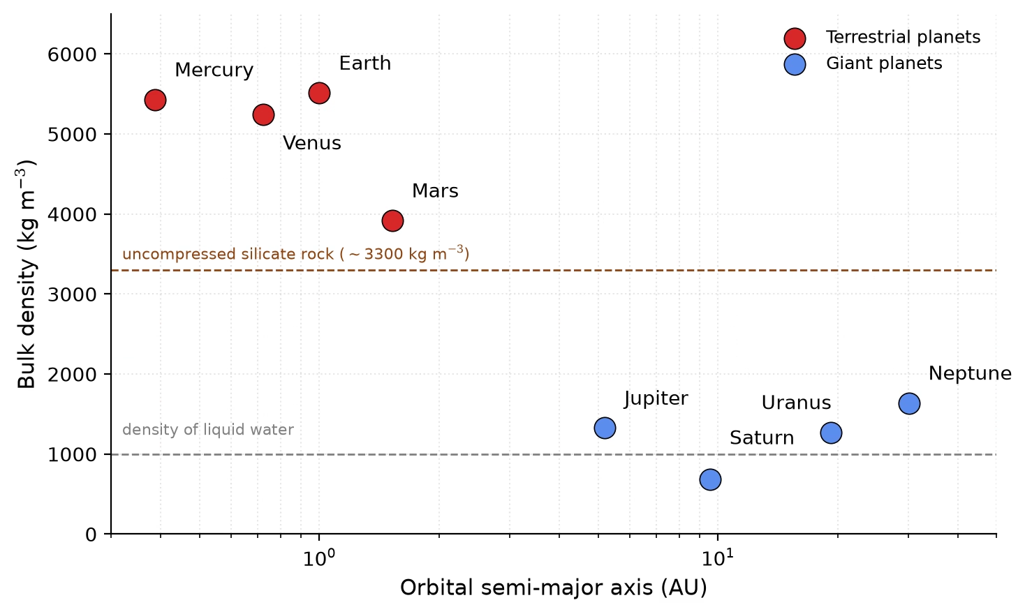
Fig. 1.16 Bulk density of the eight solar-system planets versus orbital semi-major axis (log \(x\)). The terrestrial planets (red) cluster at \(\rho > 3900\) kg m\(^{-3}\); the giant planets (blue) sit below 1700 kg m\(^{-3}\), with Saturn the lowest at 687 kg m\(^{-3}\), below the density of liquid water (grey dashed line). The tan dashed line marks the uncompressed density of typical silicate mantle rock (\(\sim 3300\) kg m\(^{-3}\), the 1-bar density of olivine and peridotite): Mars sits close to this value, while Earth, Venus, and Mercury exceed it because (a) iron-rich cores raise the bulk density and (b) self-gravity compresses their interiors. The formation context of this density gradient is developed in Lecture 2. Data from [NASA Jet Propulsion Laboratory, 2026]. Course-original figure.

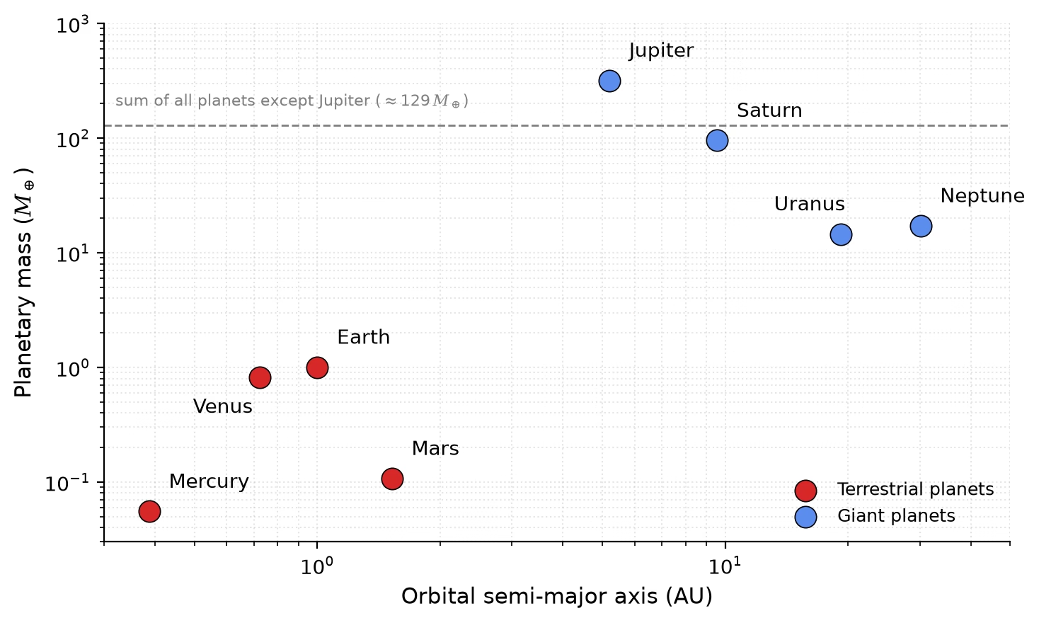
Fig. 1.17 Planetary mass versus orbital semi-major axis on a log-log scale, on the same x-axis as Fig. 1.16. The grey dashed line marks the sum of all planetary masses except Jupiter (\(\approx 129\,\Mearth\)); Jupiter alone, at \(317.83\,\Mearth\), exceeds this sum by a factor of \(\approx 2.5\) and sits well above the line. Jupiter and Saturn together account for more than \(90\%\) of the total planetary mass in the solar system. The formation context of this mass concentration is developed in Lecture 2. Data from [NASA Jet Propulsion Laboratory, 2026]. Course-original figure.

1.4.3. Classification

Planets are broadly classified by composition and structure:

• Terrestrial planets (Mercury, Venus, Earth, Mars): Rocky surfaces, iron cores, thin or no atmospheres (Venus being the exception with its massive CO\(_2\) atmosphere). Covered in Lecture 9 and Lecture 10.

• Gas giants (Jupiter, Saturn): Massive hydrogen-helium envelopes with no well-defined solid surface, likely rocky/icy cores at high pressure. Covered in Lecture 11.

• Ice giants (Uranus, Neptune): Smaller than gas giants, with interiors dominated by heavier volatiles (H\(_2\)O, NH\(_3\), CH\(_4\)) under extreme pressures, topped by hydrogen-helium atmospheres. Also covered in Lecture 11.

1.5. Blackboard derivation: Solar mass from planetary orbits

Blackboard derivation: Solar mass from Kepler’s third law

Goal: Use Kepler’s third law to estimate the mass of the Sun from Earth’s orbital parameters, then evaluate the planet-to-star mass ratio for the solar system.

Setup.

Consider a planet of mass \(M_p\) in a circular orbit of radius \(r\) around a star of mass \(M_*\). The gravitational force provides the centripetal acceleration:

\[ \frac{G M_* M_p}{r^2} = \frac{M_p v^2}{r} \]

where \(v = 2\pi r / P\) is the orbital velocity and \(P\) is the orbital period.

Derivation.

Substituting \(v = 2\pi r / P\) and cancelling \(M_p\):

\[ \frac{G M_*}{r^2} = \frac{4\pi^2 r}{P^2} \]

Solving for the stellar mass:

\[ \boxed{M_* = \frac{4\pi^2 r^3}{G P^2}} \]

This is Newton’s form of Kepler’s third law (for \(M_p \ll M_*\)). The planet’s mass cancels: the orbital period depends only on the central mass and the orbital radius.

Note: For elliptical orbits, the same relation holds with \(r\) replaced by the semi-major axis \(a\). The derivation of the general case requires the vis-viva equation, which we will cover in Lecture 2.

Application.

Using Earth’s orbital parameters:

Quantity	Value
Semi-major axis \(a_\oplus\)	\(1.496 \times 10^{11}\) m
Orbital period \(P_\oplus\)	\(3.156 \times 10^7\) s
Gravitational constant \(G\)	\(6.674 \times 10^{-11}\) m\(^3\) kg\(^{-1}\) s\(^{-2}\)

\[ \Msun = \frac{4\pi^2 \times (1.496 \times 10^{11})^3}{6.674 \times 10^{-11} \times (3.156 \times 10^7)^2} \approx 1.99 \times 10^{30} \text{ kg} \]

This agrees with the accepted value \(\Msun = 1.989 \times 10^{30}\) kg, a remarkably accurate estimate from just two measurable quantities.

The planet-to-star mass ratio.

The more precise form of Kepler’s third law is \(P^2 = 4\pi^2 a^3 / [G(M_* + M_p)]\), which gives \(M_* + M_p\) rather than \(M_*\) alone. The approximation \(M_* + M_p \approx M_*\) is justified because the planet-to-star mass ratio is tiny:

• Jupiter, the most massive planet: \(\Mjup \approx 318 \, \Mearth \approx 1.90 \times 10^{27}\) kg, giving \(\Mjup / \Msun \approx 9.5 \times 10^{-4}\).

• Total mass of all eight planets: \(\approx 446 \, \Mearth \approx 2.7 \times 10^{27}\) kg, giving \(M_\mathrm{planets}/\Msun \approx 1.3 \times 10^{-3}\).

The Sun contains 99.87% of the solar system’s total mass. Jupiter alone accounts for 71% of the planetary mass (Fig. 1.18). This extreme concentration of mass in the central star is a fundamental property of planetary systems, and one that planet formation theory must explain (Lecture 2).

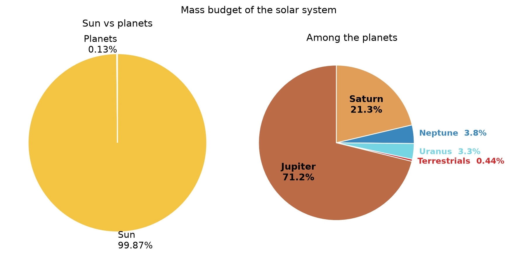
Fig. 1.18 Mass budget of the solar system. Left: the Sun contains 99.87% of the total mass; the eight planets together contribute the remaining 0.13%. Right: among the planets, Jupiter accounts for \(\sim 71\%\) and Saturn \(\sim 21\%\); the ice giants Neptune (\(3.8\%\)) and Uranus (\(3.3\%\)) make up most of the rest; the four terrestrial planets (Mercury, Venus, Earth, Mars) together contribute only \(0.44\%\) of the planetary mass and are grouped into a single wedge for legibility. Data from [NASA Jet Propulsion Laboratory, 2026]. Course-original figure.

1.6. Comparative planetology as a methodology

Understanding a single planet in isolation is difficult: we cannot perform controlled experiments on entire worlds. Comparative planetology addresses this by treating the planets as a natural set of experiments: similar objects subjected to different conditions.

Consider the terrestrial planets (Fig. 1.19). Venus, Earth, and Mars have broadly similar compositions and formed in the same protoplanetary disk, yet their surfaces and atmospheres are radically different:

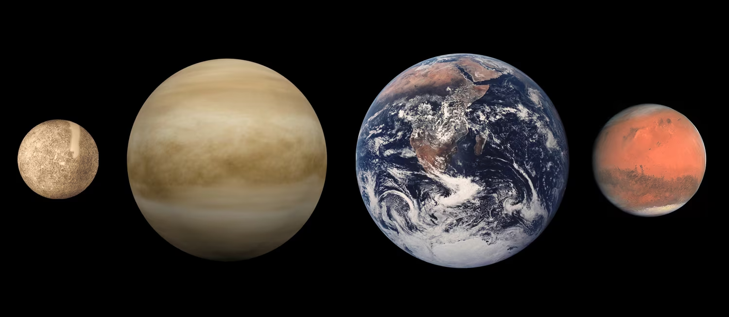
Fig. 1.19 The four terrestrial planets at approximate relative scale. From left to right: Mercury, Venus, Earth, and Mars. Despite forming in the same protoplanetary disk, these worlds span a factor of about 18 in mass and have followed dramatically different evolutionary paths. Earth and Venus are studied in detail in Lecture 9; Mercury and Mars in Lecture 10. Credit: NASA/JPL, public domain.

Property	Venus	Earth	Mars
Surface temperature	464 °C	15 °C	\(-63\) °C
Surface pressure	92 bar	1 bar	0.006 bar
Dominant atmosphere	CO\(_2\) (96.5%)	N\(_2\)/O\(_2\) (99%)	CO\(_2\) (95%)
Magnetic field	None	Strong dipole	Remnant crustal
Tectonics	Episodic resurfacing	Plate tectonics	Stagnant lid

The atmospheric divergence is striking: Fig. 1.20 shows that the three planets span four orders of magnitude in surface pressure and several hundred kelvin in surface temperature.

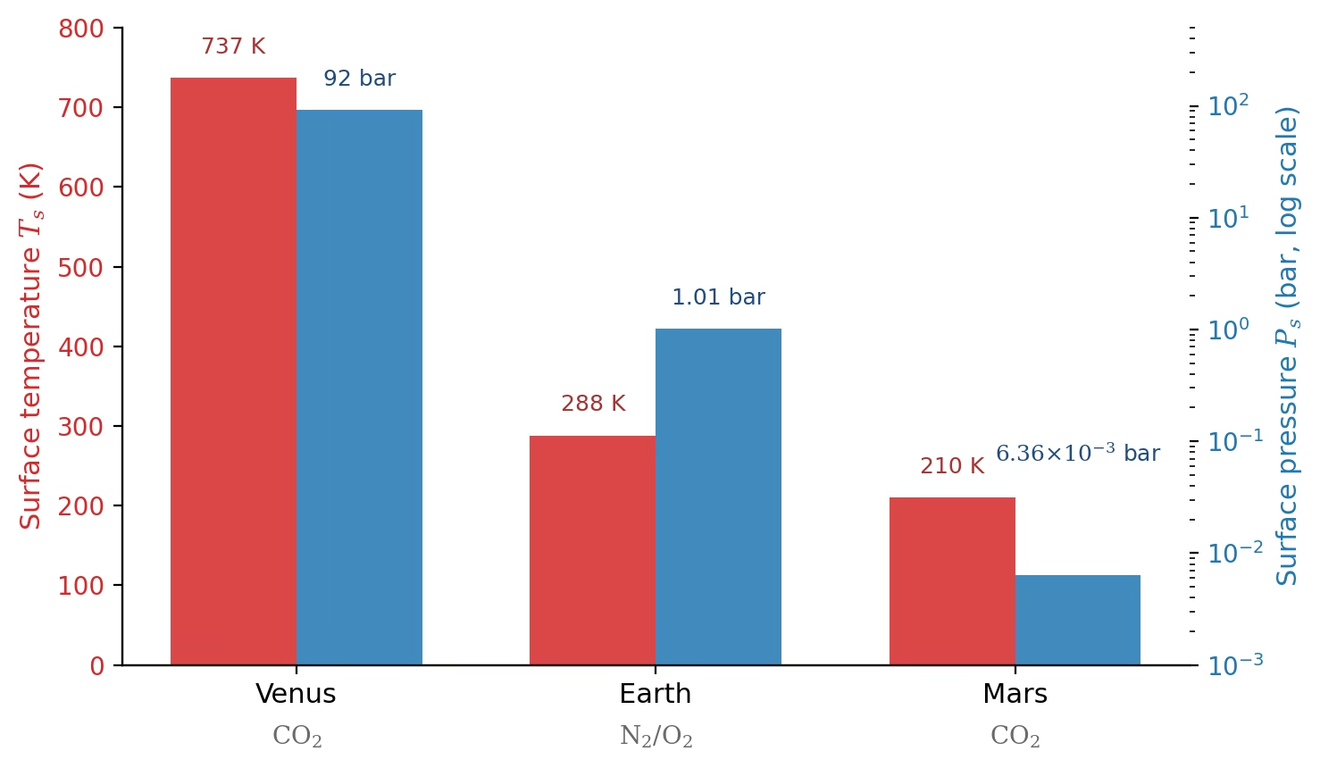
Fig. 1.20 Surface temperature (red bars, left axis) and surface pressure (blue bars, right axis, log scale) for Venus, Earth, and Mars, with the dominant atmospheric species labelled below. Despite similar bulk compositions and shared formation environment, the three terrestrial planets span a factor of \(\sim 10^4\) in surface pressure and \(\sim 500\) K in surface temperature. Data from [NASA Jet Propulsion Laboratory, 2026]. Course-original figure.

By comparing these three cases, we can isolate which differences arise from distance to the Sun, planetary mass, internal activity, or historical contingency. The same logic applies to moons: comparing Io, Europa, Ganymede, and Callisto (Fig. 1.21), all orbiting Jupiter but differing in composition and tidal heating, reveals how a single variable can drive vastly different geological outcomes.

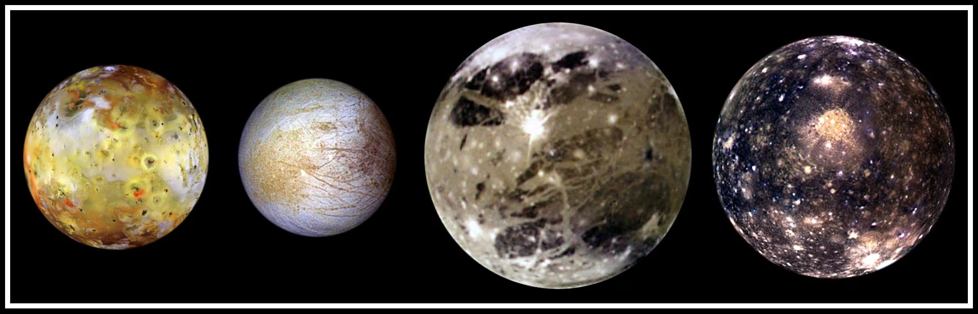
Fig. 1.21 The four Galilean moons of Jupiter at correct relative size. Left to right: Io (volcanically active), Europa (icy crust over a global liquid-water ocean), Ganymede (largest moon in the solar system at 5262 km in diameter, larger than Mercury at 4880 km; intrinsic magnetic field), Callisto (heavily cratered, geologically inert). Despite a common formation environment, tidal heating and ice content drive vastly different geological outcomes; the giant-planet moon systems are revisited in Lecture 11. Credit: NASA/JPL/DLR, Galileo mission.

This comparative approach now extends to thousands of exoplanets, where we can study how planetary properties vary as a function of stellar type, orbital distance, and system architecture (Lecture 13). It is one of the most powerful tools in modern planetary science, and we will apply it throughout this course.

1.7. Observational techniques

Planetary science draws on a wide range of observational methods, from ground-based telescopes to robotic landers.

1.7.1. Telescopes

Ground-based telescopes observe planets across the electromagnetic spectrum. Optical imaging resolves surface and atmospheric features, infrared spectroscopy probes thermal emission and atmospheric composition, and radio observations measure subsurface properties and atmospheric dynamics. Adaptive optics on large telescopes (e.g., VLT, Keck) achieve angular resolutions approaching those of space telescopes. ESO’s Very Large Telescope (Fig. 1.22), four 8.2 m unit telescopes on Cerro Paranal in the Atacama Desert, is one of the workhorses of ground-based solar-system astronomy: SPHERE-ZIMPOL has resolved disk-integrated shapes of large main-belt asteroids, NACO and SINFONI have tracked the seasonal hazes of Titan and the storms of Saturn and Jupiter, and the VLT supported the Rosetta mission with high-cadence monitoring of comet 67P/Churyumov-Gerasimenko on approach to perihelion.

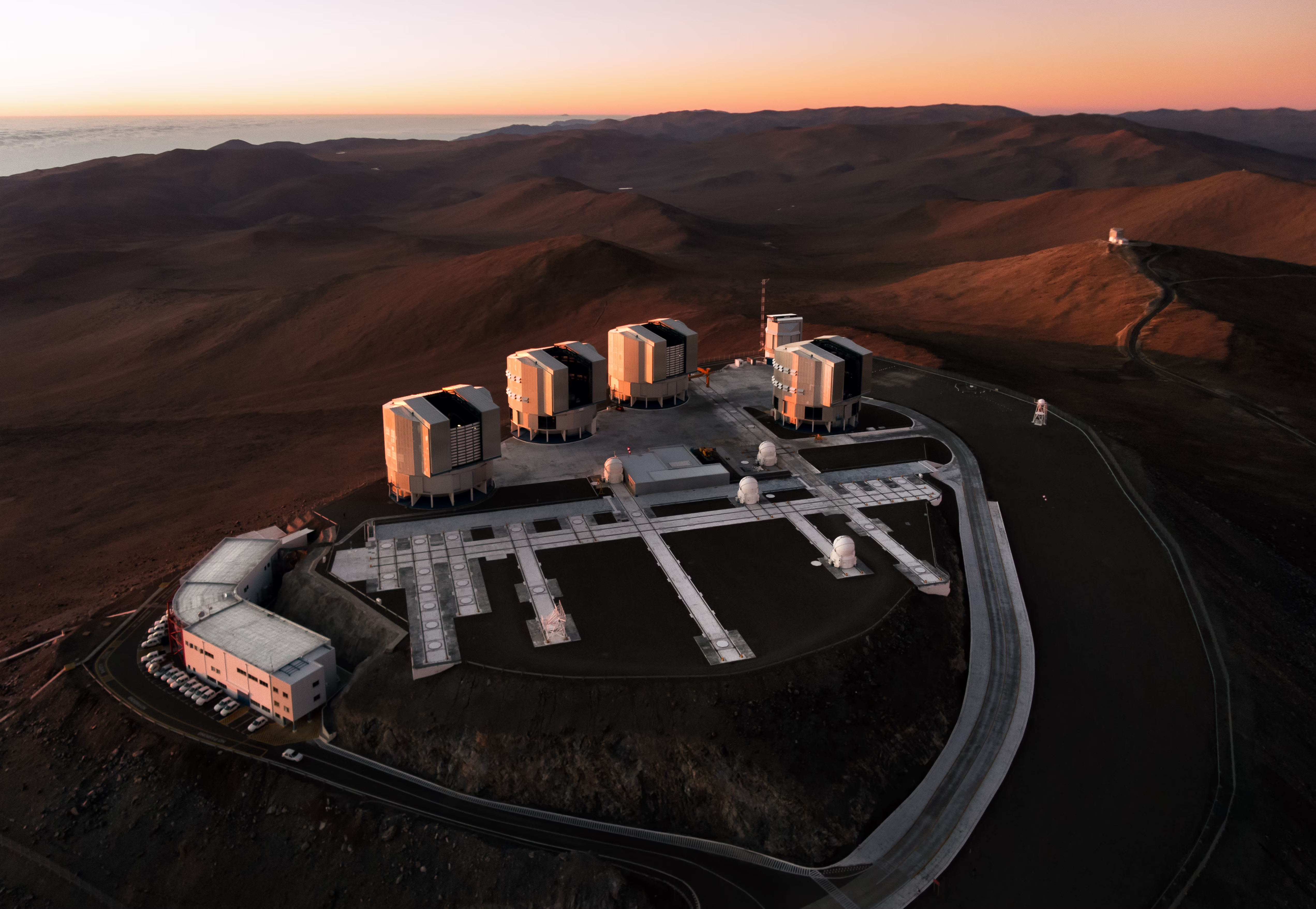
Fig. 1.22 Aerial view of ESO’s Paranal Observatory at sunset, Atacama Desert, Chile. The four 8.2 m Unit Telescopes of the Very Large Telescope (VLT) and the 4.1 m VISTA survey telescope (on an adjacent peak) are visible on the summit ridge. The dry, high-altitude site delivers some of the best optical and near-infrared seeing in the world. Image credit: G. Hüdepohl (atacamaphoto.com)/ESO [ESO, 2015].

Space-based observatories avoid atmospheric absorption and distortion. The Hubble Space Telescope (Fig. 1.23) has monitored atmospheric changes on the giant planets for decades; its Outer Planets Atmospheres Legacy (OPAL) programme has tracked Jupiter’s Great Red Spot, Saturn’s polar hexagon, and Uranus / Neptune cloud variability with annual cadence since 2014. JWST (Fig. 1.24), operating at infrared wavelengths from the Sun-Earth L2 point, is now the primary tool for exoplanet atmospheric characterisation; the carbon-dioxide detection in WASP-39 b (Fig. 1.14) and the thermal emission of TRAPPIST-1 b (Fig. 1.30) are early examples.

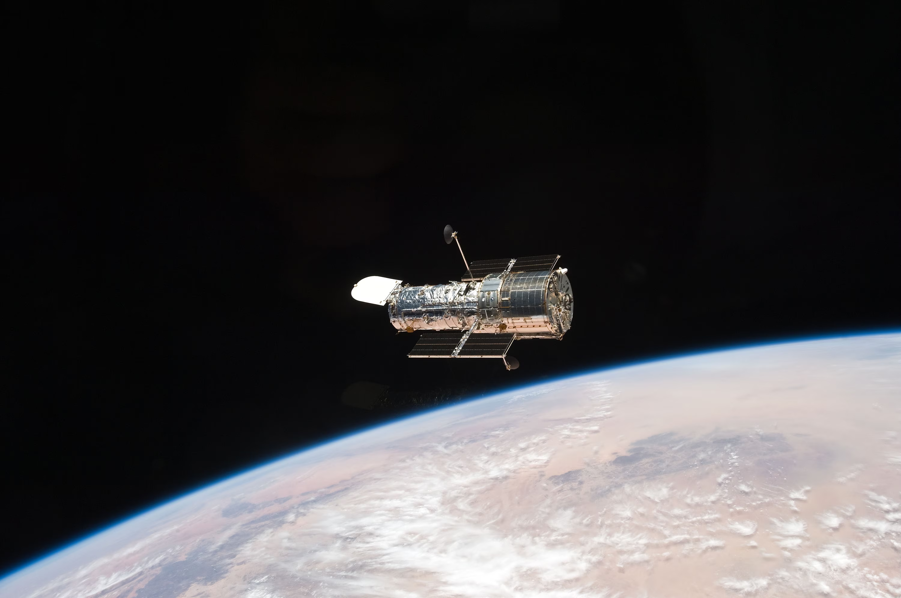
Fig. 1.23 The Hubble Space Telescope photographed from Space Shuttle Atlantis on 19 May 2009, immediately after release at the end of Servicing Mission 4 (STS-125). Five servicing missions between 1993 and 2009 extended Hubble’s lifetime by replacing instruments, gyroscopes, batteries, and solar arrays; SM4 added Wide Field Camera 3 and the Cosmic Origins Spectrograph, both still operating today. Image credit: NASA [NASA, 2009].

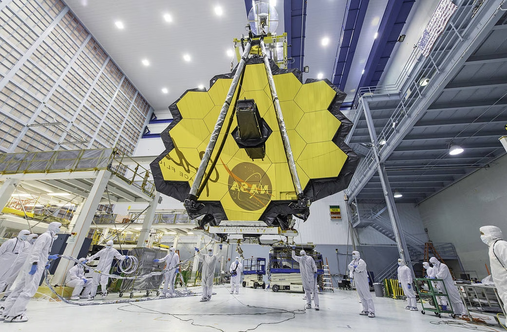
Fig. 1.24 The James Webb Space Telescope’s 6.5 m primary mirror, made of 18 gold-coated beryllium hexagons, fully deployed in a clean room at NASA’s Goddard Space Flight Center in April 2017 prior to launch. JWST observes from the Sun-Earth L2 Lagrange point, 1.5 million km from Earth, and combines a \(\sim 25 \mathrm{\,m^2}\) collecting area with cryogenic (\(T < 50\) K) optics optimised for near- and mid-infrared spectroscopy of exoplanet atmospheres. Image credit: NASA / D. Stover [NASA, 2017].

1.7.2. Spacecraft exploration

Spacecraft provide the most detailed planetary data. NASA’s currently active and planned planetary missions are summarised in Fig. 1.25, ranging from the Voyagers in interstellar space and Juno at Jupiter to the New Frontiers (OSIRIS-APEX, Dragonfly), Discovery (Lucy, Psyche, DAVINCI, VERITAS), and Mars program assets (Perseverance + Ingenuity, Curiosity, MAVEN, Mars Reconnaissance Orbiter, the InSight legacy data set). The European counterpart (Fig. 1.26) has been built up over four decades from Giotto’s 1986 Halley flyby through current missions (BepiColombo at Mercury, Mars Express, the Jupiter Icy Moons Explorer JUICE en route to the Jupiter system) and into the planned EnVision Venus orbiter and the Comet Interceptor that will wait at L2 for a target.

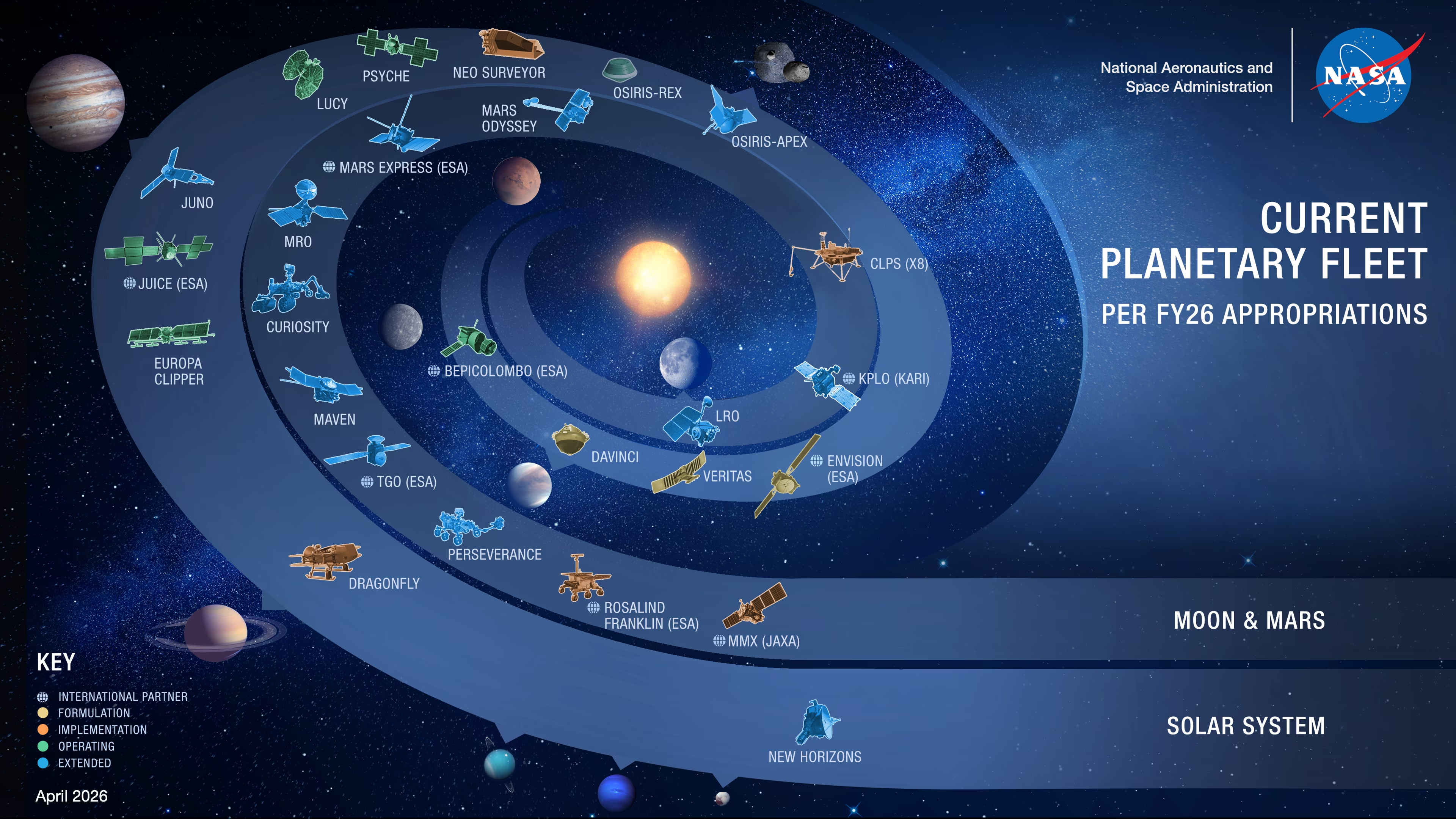
Fig. 1.25 NASA’s current planetary fleet, per the FY26 appropriations, organised by target (inner Solar System, Mars, asteroids and small bodies, outer planets, heliopause). Status May 2026; bodies and orbits are not to scale. The poster reflects budgeted mission state and therefore omits a few extended-mission and concept-stage projects that may still be active. Image credit: NASA Scientific Visualization Studio / Goddard Space Flight Center; graphics by J. Mottar [NASA Scientific Visualization Studio, 2026].

Fig. 1.26 ESA’s past, present, and future Solar System exploration missions (status September 2025). Planetary highlights include Giotto at Halley (1986), the Cassini-Huygens partnership (Huygens landed on Titan in 2005), Rosetta and Philae at comet 67P/Churyumov-Gerasimenko (2014-2016), Venus Express (2006-2014), Mars Express (2003-active), BepiColombo (en route to Mercury), JUICE (en route to the Jupiter system), and the upcoming EnVision Venus orbiter, ExoMars Rosalind Franklin rover, and Comet Interceptor. The poster also labels several lunar and heliospheric missions (Ulysses, SOHO, SMART-1, Chandrayaan-1, Solar Orbiter, Proba-2/3, MMX) that contribute to the broader Solar System exploration programme but lie outside the planetary highlights named here. Image credit: ESA (CC BY-SA 3.0 IGO) [ESA, 2025].

Mission types include, in order of increasing complexity and cost:

• Flyby: The spacecraft passes a target once, collecting data during a brief encounter. Example: Voyager 2 at Neptune (1989).

• Orbiter: The spacecraft enters orbit, enabling long-term monitoring. Example: Cassini at Saturn (2004 to 2017).

• Lander: The spacecraft lands on the surface and measures conditions in situ. Example: Viking 1 on Mars (1976).

• Rover: A mobile lander that traverses the surface. Example: Perseverance on Mars (2021 to present).

• Sample return: Material is collected and returned to Earth for laboratory analysis. Example: Hayabusa2 returned samples from asteroid Ryugu (2020).

1.7.3. Remote sensing methods

Key remote sensing techniques used across these platforms include:

• Spectroscopy: Identifies materials by their characteristic absorption and emission features. Reveals atmospheric composition, surface mineralogy, and thermal properties.

• Radar: Penetrates clouds and maps surface topography (e.g., Magellan at Venus) and detects subsurface features (e.g., MARSIS on Mars).

• Gravimetry: Maps the gravity field from spacecraft orbital perturbations, revealing interior density variations and subsurface mass concentrations.

• Magnetometry: Measures magnetic fields, constraining dynamo activity and interior conductivity.

1.8. Key spacecraft missions

The table below lists landmark missions that have shaped our understanding of the solar system.

Selected landmark planetary missions.

Mission	Agency	Year(s)	Target	Key achievement
Mariner 2	NASA	1962	Venus	First successful planetary flyby
Mariner 4	NASA	1965	Mars	First close-up images of another planet
Apollo 11	NASA	1969	Moon	First crewed landing on another world
Venera 7	USSR	1970	Venus	First successful landing on another planet
Viking 1 & 2	NASA	1976	Mars	First Mars landers; life-detection experiments
Voyager 1 & 2	NASA	1977-1989	Outer planets	Grand tour of Jupiter, Saturn, Uranus, Neptune
Giotto	ESA	1986	Comet 1P/Halley	First close-up images of a comet nucleus
Galileo	NASA	1995-2003	Jupiter	First Jupiter orbiter; Europa’s subsurface ocean
Mars Express	ESA	2003-	Mars	First ESA planetary orbiter; subsurface water-ice detection
Cassini-Huygens	NASA/ESA	2004-2017	Saturn	Huygens landed on Titan; Enceladus plumes
Spirit & Opportunity	NASA	2004-2018	Mars	Long-duration rovers; evidence for past water
Venus Express	ESA	2006-2014	Venus	Long-term monitoring of the Venusian atmosphere
Rosetta / Philae	ESA	2014-2016	Comet 67P	First comet orbiter; Philae made the first comet landing
New Horizons	NASA	2015	Pluto	First Pluto flyby; revealed geological complexity
Hayabusa2	JAXA	2014-2020	Ryugu	Returned samples from a carbonaceous asteroid
Juno	NASA	2016-2025	Jupiter	First Jupiter polar orbiter; interior structure from gravity and magnetic mapping
BepiColombo	ESA/JAXA	2018-	Mercury	Two-orbiter mission; Mercury orbit insertion November 2026
Perseverance	NASA	2021-	Mars	Sample caching for future return; Ingenuity helicopter
JWST	NASA/ESA/CSA	2021-	Exoplanets	Atmospheric characterisation of exoplanets
Chang’e 6	CNSA	2024	Moon (far side)	First samples returned from the lunar far side
Europa Clipper	NASA	2024-	Europa	Investigating habitability of Europa’s ocean

Two iconic mission products illustrate the breadth of these efforts: the Cassini orbiter’s backlit view of Saturn from inside the planet’s shadow (Fig. 1.27), and the first colour view from Perseverance on Mars (Fig. 1.28) showing the rocky plain in Jezero crater where samples for eventual return are being cached.

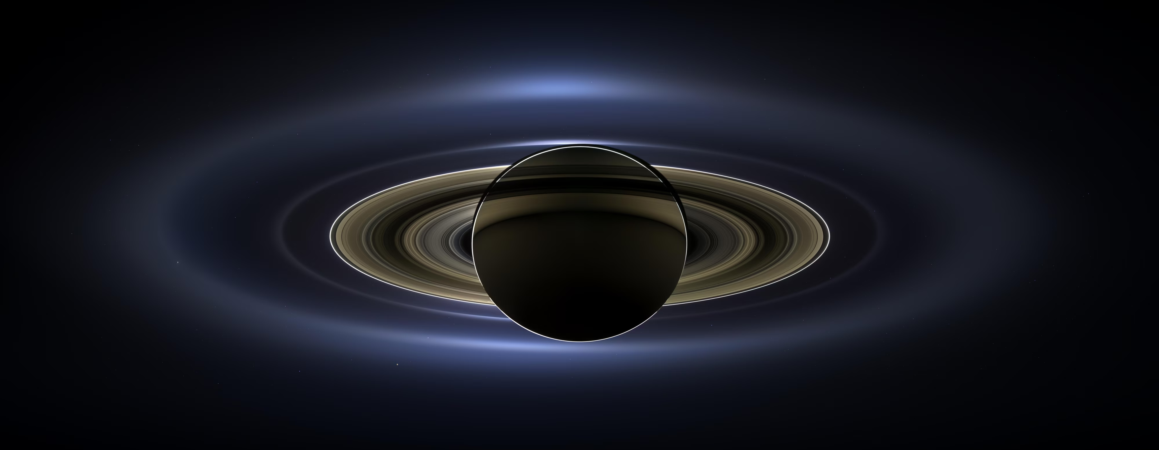
Fig. 1.27 Backlit view of Saturn imaged by the Cassini spacecraft on 19 July 2013 from inside the planet’s shadow, with Earth visible as a faint pale point through the rings (lower right). The image is known as “The Day the Earth Smiled” because it is the first Earth portrait from deep space that was pre-announced to the public; Voyager 1’s Pale Blue Dot (Fig. 1.1) and the Voyager Family Portrait (Fig. 1.2) were imaged without public advance notice. Cassini operated in Saturn orbit from 2004 to 2017 and discovered the global subsurface ocean of Enceladus and the hydrocarbon lakes of Titan; Saturn’s rings, Enceladus, and Titan are returned to in Lecture 11. Credit: NASA/JPL-Caltech/Space Science Institute.

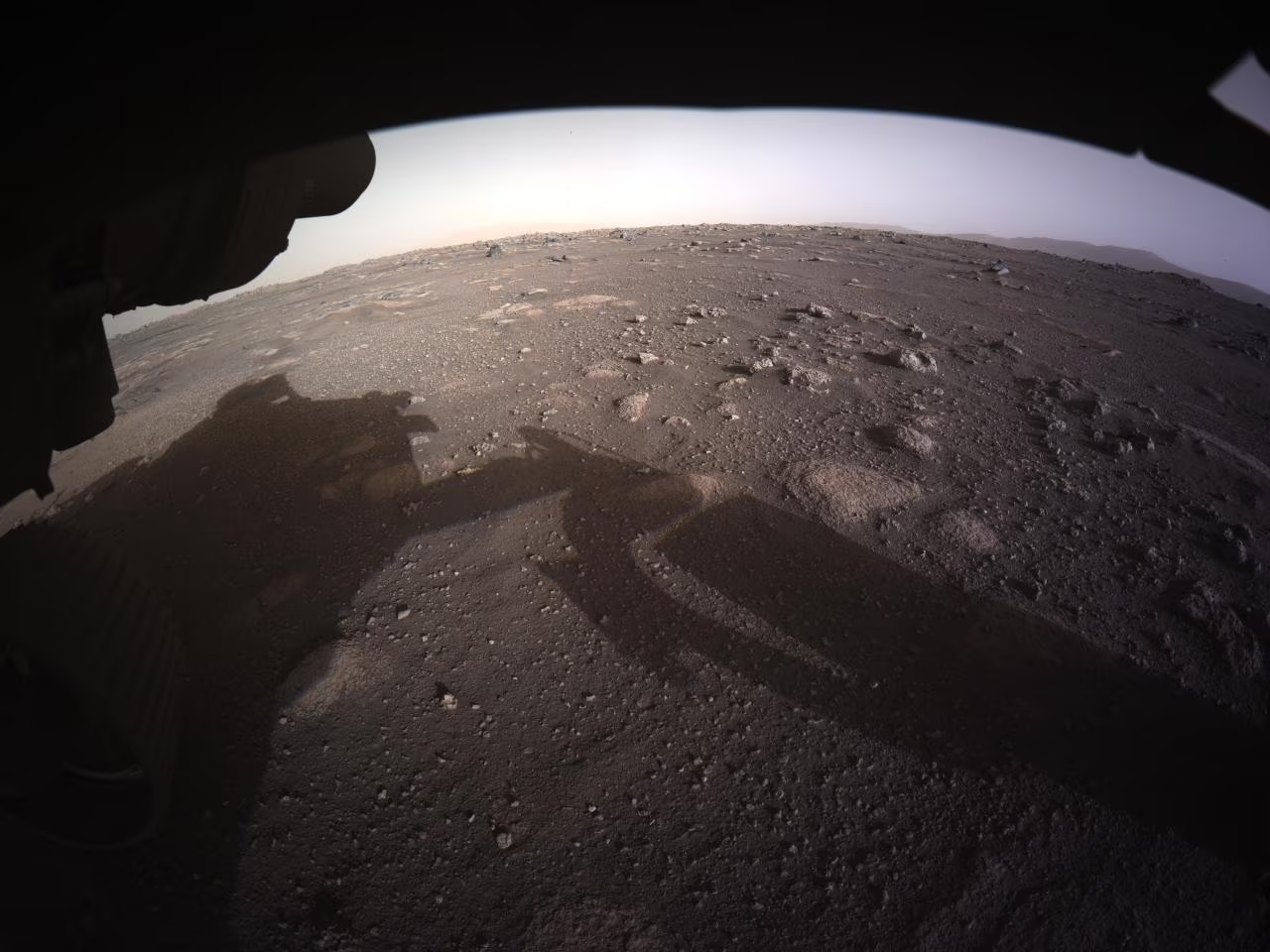
Fig. 1.28 First colour view of Mars from NASA’s Perseverance rover, taken from one of its hazard-avoidance cameras shortly after landing in Jezero crater on 18 February 2021. The rover’s shadow and parts of its body are visible in the foreground; the rocky plain ahead is part of an ancient lake-delta system that filled Jezero crater during the Noachian (Mars’s earliest geological era), around 3.6 Ga ago. Perseverance is caching rock and regolith samples for return to Earth via the Mars Sample Return campaign, whose return architecture is currently being re-baselined; Jezero stratigraphy, the Mars climate history, and the sample-return programme are returned to in Lecture 10. Credit: NASA/JPL-Caltech.

Several missions are in flight or planned for the coming decade, including ESA’s JUICE (launched April 2023, Jupiter system arrival 2031, Ganymede orbit insertion 2034), the Mars Sample Return campaign, and the Dragonfly rotorcraft to Titan (launch ~2028).

1.9. Recent advances

Planetary science is advancing rapidly, driven by new space missions and observatories. JWST, launched in 2021, has begun characterising the atmospheres of rocky exoplanets for the first time, including thermal emission measurements of planets in the TRAPPIST-1 system [Greene et al., 2023] (see also Lecture 13). The system architecture, with seven roughly Earth-sized planets in tightly-packed orbits around a ultra-cool dwarf star, is shown in Fig. 1.29. These observations are providing the first direct constraints on whether Earth-sized planets around other stars retain atmospheres; the first such measurement, the dayside thermal emission of TRAPPIST-1 b, is shown in Fig. 1.30.

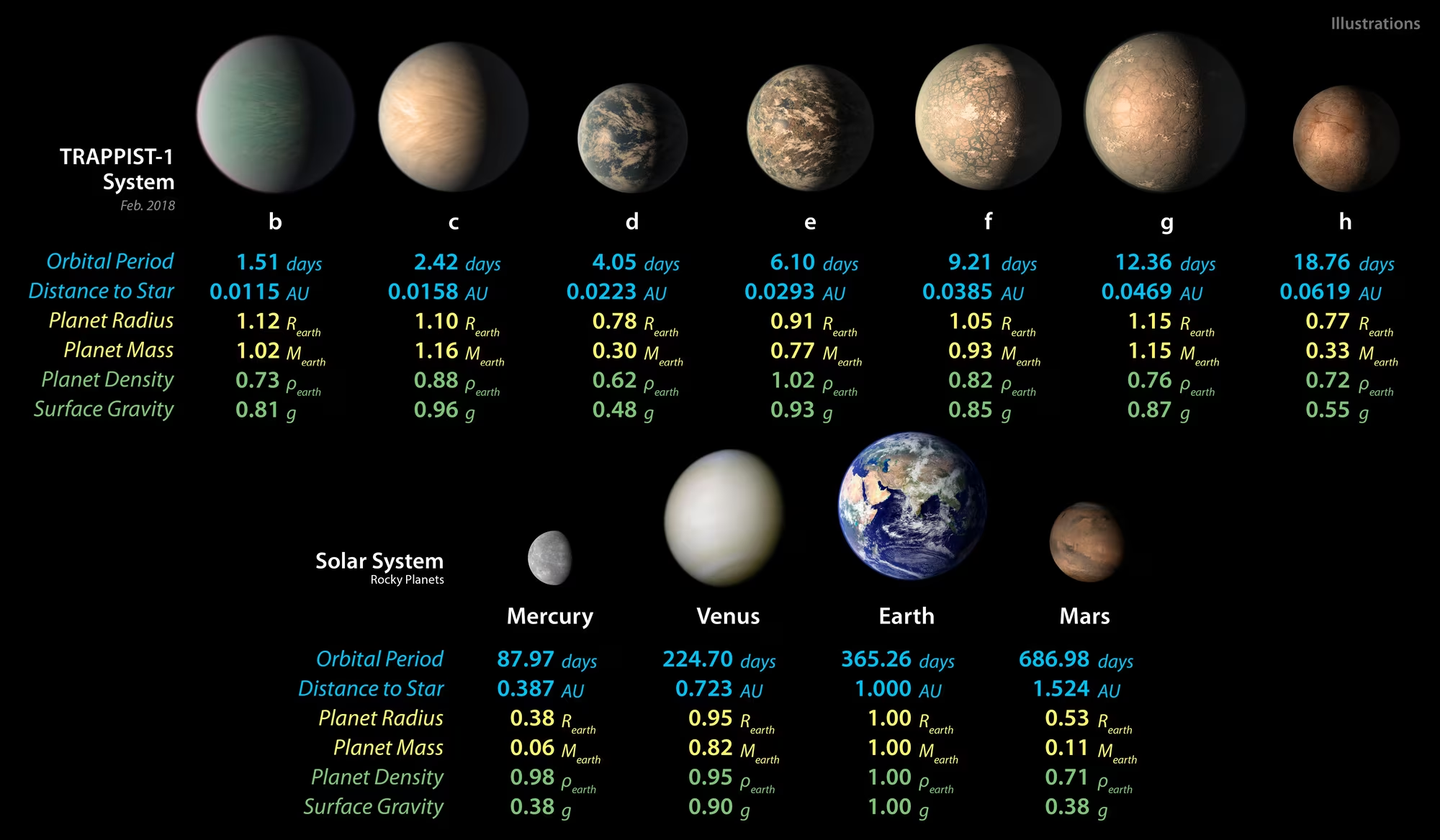
Fig. 1.29 The seven planets of the TRAPPIST-1 system (top row, b through h) compared with the inner solar system (bottom row), shown with measured or estimated orbital periods, distances, radii, masses, densities, and surface gravities. All seven TRAPPIST-1 planets are roughly Earth-sized and orbit closer to their ultra-cool dwarf star host than Mercury does to the Sun: their orbital periods range from 1.5 days (b) to 19 days (h), so the entire system fits well inside Mercury’s 88-day orbit. The seven planets sit in a chain of six mean-motion resonances [Gillon et al., 2017, Luger et al., 2017] that locks the orbital periods into integer ratios; three planets (e, f, g) are inside the conservative habitable zone and a fourth (d) sits near its inner edge. The planet renderings in the top row are artist’s illustrations, not telescope images: TRAPPIST-1 lies \(\sim 12\) pc from Earth and its planets are far too small and faint to be spatially resolved with current instruments, while the bottom-row inner solar system images are spacecraft photographs. Credit: NASA/JPL-Caltech.

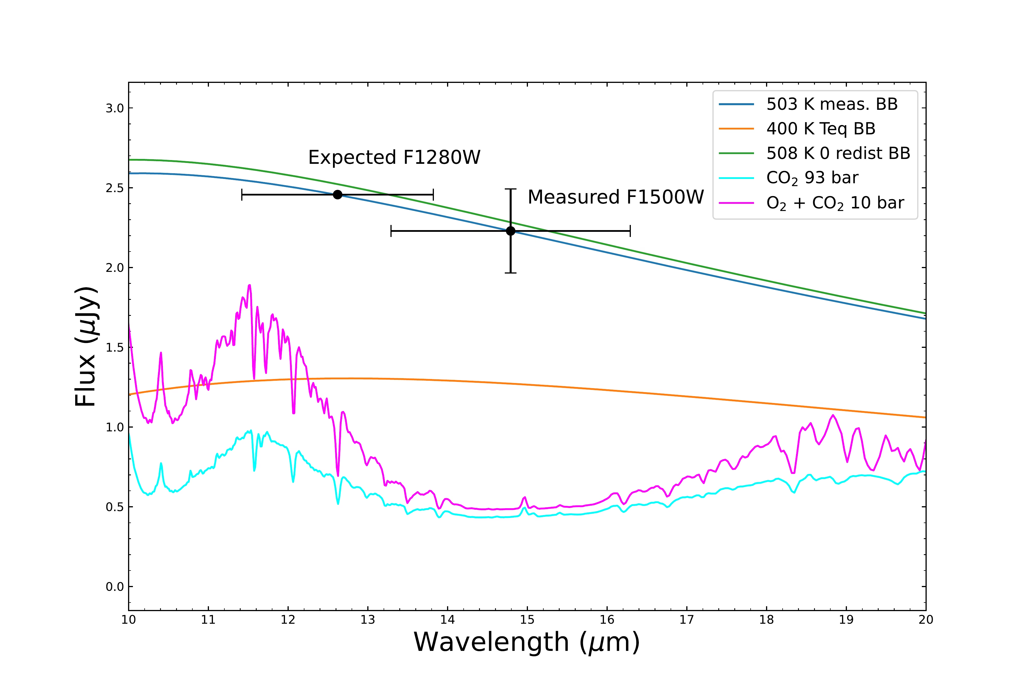
Fig. 1.30 JWST F1500W secondary-eclipse measurement of TRAPPIST-1 b with the Mid-Infrared Instrument (MIRI): the first thermal measurement of a rocky exoplanet around an M dwarf. The horizontal axis is wavelength in microns; the vertical axis is the planet’s spectral flux density in microjanskys (μJy). The two black points with error bars are JWST MIRI photometric measurements: the F1280W band centred on 12.8 μm (labelled Expected, the value the planet would emit if it followed the measured 15-μm dayside blackbody) and the F1500W band centred on 15 μm (labelled Measured, the secondary-eclipse depth that gives the actual planet emission at that wavelength). Five model curves are overplotted: three blackbody predictions (blue: \(503 \pm 27\) K dayside brightness temperature; orange: 400 K equilibrium temperature with full heat redistribution; green: 508 K bare-rock prediction for zero heat redistribution and zero albedo) and two thick-atmosphere models (cyan: a 93-bar \(\mathrm{CO_2}\)-dominated atmosphere; magenta: a 10-bar \(\mathrm{O_2}+\mathrm{CO_2}\) atmosphere). \(\mathrm{CO_2}\) absorbs strongly near 15 μm, so the atmospheric models predict sharply suppressed flux there. The F1500W point sits on the bare-rock blackbody and well above the two atmospheric models, ruling out thick \(\mathrm{CO_2}\)-rich atmospheres on TRAPPIST-1 b and indicating that the planet retains little or no thick atmosphere. The atmospheric retention of M-dwarf rocky planets is the central question this kind of measurement is built to answer, treated in detail in Lecture 13. Reproduced from Greene et al. [2023].

Closer to home, NASA’s OSIRIS-REx mission returned samples from the carbon-rich asteroid Bennu in September 2023, revealing hydrated minerals and organic compounds that illuminate the primordial building blocks of planets (Lecture 12). The moment of sample acquisition is shown in Fig. 1.31: the spacecraft’s TAGSAM head (Touch-and-Go Sample Acquisition Mechanism) pressed into Bennu’s surface for six seconds, fired a burst of nitrogen gas to mobilise the regolith, and then backed away.

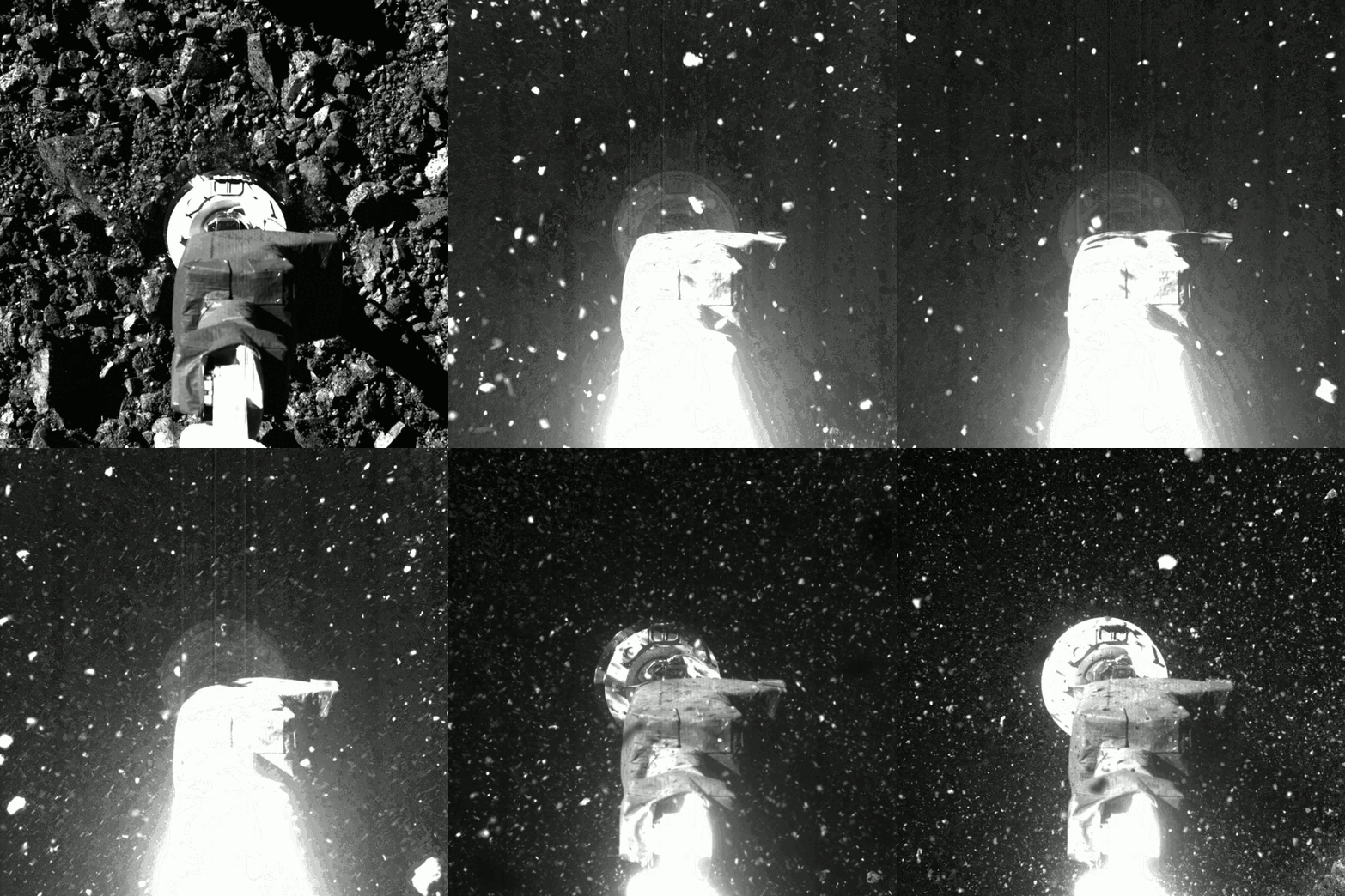
Fig. 1.31 NASA’s OSIRIS-REx spacecraft samples asteroid Bennu, 20 October 2020 (animation; refresh the page if it is not playing). The SamCam imager recorded the Touch-and-Go (TAG) event at sample site Nightingale from initial approach through touch-down and back-away. The TAGSAM sampling head visibly crushes the porous surface regolith on contact; the bright pulse one second after contact is the nitrogen-gas jet that mobilised the material later captured for return to Earth. The mission returned 121.6 g of pristine asteroid material to the Utah Test and Training Range on 24 September 2023, the largest asteroid sample ever brought to Earth. Asteroids and small bodies are returned to in Lecture 12. Credit: NASA / Goddard / University of Arizona [NASA, 2020].

The Mars exploration programme continues with the Perseverance rover caching samples in Jezero crater for return to Earth [Farley et al., 2022] (subject to the ongoing rebaselining of the Mars Sample Return architecture, Lecture 10), and NASA’s Dragonfly rotorcraft, a nuclear-powered drone that will explore Titan’s surface chemistry, is planned for launch in 2028 and arrival in 2034 (Lecture 11, Lecture 14).

1.10. The three central questions of this course

The bodies, missions, and measurements introduced in this lecture set up three driving questions that organise the remaining thirteen lectures. The course is structured so that each question is answered piece by piece, returning to the same set of objects, but viewed through a sharper instrument each time.

1. How do planetary systems form? The mass concentration in Jupiter and Saturn (Fig. 1.18), the dust gaps imaged by ALMA in HL Tau (Fig. 1.13), and the small-planet radius valley in Fig. 1.12 are all clues about a process we cannot watch in real time: how a collapsing molecular cloud becomes a star surrounded by a disk, how dust grows by ten orders of magnitude in size into planetesimals and protoplanets, and how the resulting bodies are sorted by gas drag, gravitational scattering, and resonances into the orbital architecture we see today. Lecture 2 introduces the disk picture and the orbital dynamics; Lecture 3 follows the energy budget of accretion and short-lived radionuclides; Lecture 12 returns to the small bodies (asteroids, comets, Kuiper-belt objects) that preserve the formation epoch in their compositions.

2. What makes a planet habitable? Venus, Earth, and Mars formed from broadly the same building blocks at broadly similar heliocentric distances, and yet they span four orders of magnitude in surface pressure and 500 K in surface temperature (Fig. 1.20). The reasons are coupled rather than independent: planetary interiors and dynamos (Lecture 4, Lecture 8) set the rate at which heat and volatiles leak out of the deep planet; atmospheres and climate (Lecture 5, Lecture 6) determine surface temperature, the rate of escape to space, and the chemistry available at the surface; surface processes (Lecture 7) close the cycle by returning volatiles to the interior. The case studies in Lecture 9 (Earth and Venus) and Lecture 10 (Mercury and Mars) put numbers on each ingredient and explain why the three inner planets diverged.

3. Does life exist beyond Earth? This is the question that motivates much of the current mission queue: JWST’s atmospheric spectra of rocky M-dwarf planets, exemplified by Fig. 1.30; JUICE and Europa Clipper at the icy moons; Dragonfly at Titan; the Extremely Large Telescope (ELT), Giant Magellan Telescope (GMT), and Thirty Meter Telescope (TMT) for direct imaging in the 2030s. Lecture 11 covers the giant planets and the ocean worlds in their moon systems. Lecture 13 places the solar system inside the exoplanet population and revisits the habitable zone. Lecture 14 closes the course on biosignatures, the Drake equation, and what the search programmes of the next two decades can and cannot answer.

1.11. Looking ahead to Lecture 2

This lecture has been a panoramic tour: the bodies, the history, the missions, and the broad outline of the discipline. The next lecture begins the actual physics. Lecture 2 walks back to the very beginning of the story, to the molecular cloud, and follows the collapse step by step: how angular momentum conservation produces a rotating disk rather than a spherical infall, how the disk’s temperature gradient sets the snow line that separates rocky from icy material, how dust grains in the disk grow by coagulation, settling, and the streaming instability to make planetesimals, and how Kepler’s laws, the vis-viva equation, and orbital resonances govern the subsequent dynamics. The history of how the solar system came to look the way it does begins not with the planets but with the disk that made them.

1.12. References

[Borucki2010]

Borucki, William J., Koch, David, Basri, Gibor, Batalha, Natalie, Brown, Timothy, Caldwell, Douglas, and others. 2010. “Kepler planet-detection mission: introduction and first results.” Science, 327(5968):977–980. doi:10.1126/science.1185402, https://ui.adsabs.harvard.edu/abs/2010Sci...327..977B/abstract.

[Brown2005] (1,2)

Brown, Michael E., Trujillo, Chadwick A., and Rabinowitz, David L. 2005. “Discovery of a planetary-sized object in the scattered Kuiper Belt.” The Astrophysical Journal, 635(1):L97–L100. doi:10.1086/499336, https://ui.adsabs.harvard.edu/abs/2005ApJ...635L..97B/abstract.

[Bryson2021] (1,2)

Bryson, Steve, Kunimoto, Michelle, Kopparapu, Ravi K., Coughlin, Jeffrey L., Borucki, William J., Koch, David, Silva Aguirre, Víctor, Allen, Christopher, Barentsen, Geert, Batalha, Natalie M., and others. 2021. “The occurrence of rocky habitable-zone planets around solar-like stars from kepler data.” The Astronomical Journal, 161(1):36. doi:10.3847/1538-3881/abc418, arXiv:2010.14812, https://ui.adsabs.harvard.edu/abs/2021AJ....161...36B/abstract.

[Farley2022]

Farley, K. A., Stack, K. M., Shuster, D. L., Horgan, B. H. N., Hurowitz, J. A., Tarnas, J. D., Simon, J. I., Sun, V. Z., Scheller, E. L., Moore, K. R., and others. 2022. “Aqueously altered igneous rocks sampled on the floor of Jezero crater, Mars.” Science, 377(6614):eabo2196. doi:10.1126/science.abo2196, https://ui.adsabs.harvard.edu/abs/2022Sci...377.2196F/abstract.

[Fulton2017]

Fulton, Benjamin J., Petigura, Erik A., Howard, Andrew W., Isaacson, Howard, Marcy, Geoffrey W., Cargile, Phillip A., Hebb, Leslie, Weiss, Lauren M., Johnson, John Asher, Morton, Timothy D., and others. 2017. “The California-Kepler Survey. III. a gap in the radius distribution of small planets.” The Astronomical Journal, 154(3):109. doi:10.3847/1538-3881/aa80eb, arXiv:1703.10375, https://ui.adsabs.harvard.edu/abs/2017AJ....154..109F/abstract.

[Gillon2017]

Gillon, Michaël, Triaud, Amaury H. M. J., Demory, Brice-Olivier, Jehin, Emmanuël, Agol, Eric, Deck, Katherine M., Lederer, Susan M., de Wit, Julien, Burdanov, Artem, Ingalls, James G., and others. 2017. “Seven temperate terrestrial planets around the nearby ultracool dwarf star TRAPPIST-1.” Nature, 542(7642):456–460. doi:10.1038/nature21360, arXiv:1703.01424, https://ui.adsabs.harvard.edu/abs/2017Natur.542..456G/abstract.

[Greene2023] (1,2)

Greene, Thomas P., Bell, Taylor J., Ducrot, Elsa, Dyrek, Achrène, Lagage, Pierre-Olivier, and Fortney, Jonathan J. 2023. “Thermal emission from the Earth-sized exoplanet TRAPPIST-1 b using JWST.” Nature, 618(7963):39–42. doi:10.1038/s41586-023-05951-7, arXiv:2303.14849, https://ui.adsabs.harvard.edu/abs/2023Natur.618...39G/abstract.

[Luger2017]

Luger, Rodrigo, Sestovic, Marko, Kruse, Ethan, Grimm, Simon L., Demory, Brice-Olivier, Agol, Eric, Bolmont, Emeline, Fabrycky, Daniel, Fernandes, Catarina S., Van Grootel, Valérie, and others. 2017. “A seven-planet resonant chain in TRAPPIST-1.” Nature Astronomy, 1:0129. doi:10.1038/s41550-017-0129, https://ui.adsabs.harvard.edu/abs/2017NatAs...1E.129L/abstract.

[Leger2009]

Léger, A., Rouan, D., Schneider, J., Barge, P., Fridlund, M., Samuel, B., Ollivier, M., Guenther, E., Deleuil, M., Deeg, H. J., and others. 2009. “Transiting exoplanets from the CoRoT space mission. VIII. CoRoT-7b: the first super-Earth with measured radius.” Astronomy & Astrophysics, 506(1):287–302. doi:10.1051/0004-6361/200911933, https://ui.adsabs.harvard.edu/abs/2009A%26A...506..287L/abstract.

[MayorQueloz1995]

Mayor, Michel and Queloz, Didier. 1995. “A Jupiter-mass companion to a solar-type star.” Nature, 378:355–359. doi:10.1038/378355a0, https://ui.adsabs.harvard.edu/abs/1995Natur.378..355M/abstract.

[Runyon2017]

Runyon, Kirby D., Stern, S. Alan, Lauer, Tod R., Grundy, Will, Summers, Michael E., and Singer, Kelsi N. 2017. “A geophysical planet definition.” In Lunar and Planetary Science Conference, volume 48, 1448. https://www.hou.usra.edu/meetings/lpsc2017/pdf/1448.pdf.

[Rustamkulov2023] (1,2)

Rustamkulov, Z., Sing, D. K., Mukherjee, S., May, E. M., Kirk, J., Schlawin, E., Line, M. R., Piaulet, C., Carter, A. L., Batalha, N. E., and others. 2023. “Early Release Science of the exoplanet WASP-39b with JWST NIRSpec PRISM.” Nature, 614(7949):659–663. doi:10.1038/s41586-022-05677-y, arXiv:2211.10487, https://ui.adsabs.harvard.edu/abs/2023Natur.614..659R/abstract.

[Sagan1994]

Sagan, Carl. 1994. Pale Blue Dot: A Vision of the Human Future in Space. Random House, New York.

[Wolszczan1992]

Wolszczan, Aleksander and Frail, Dale A. 1992. “A planetary system around the millisecond pulsar PSR1257+12.” Nature, 355:145–147. doi:10.1038/355145a0, https://ui.adsabs.harvard.edu/abs/1992Natur.355..145W/abstract.

[ALMAPartnership2015]

ALMA Partnership, Brogan, C. L., Pérez, L. M., Hunter, T. R., Dent, W. R. F., Hales, A. S., Hills, R. E., Corder, S., Fomalont, E. B., Vlahakis, C., and others. 2015. “The 2014 ALMA long baseline campaign: first results from high angular resolution observations toward the HL Tau region.” The Astrophysical Journal Letters, 808(1):L3. doi:10.1088/2041-8205/808/1/L3, https://ui.adsabs.harvard.edu/abs/2015ApJ...808L...3A/abstract.

[ESAFleet2025]

ESA. 2025. Esa's science fleet of solar system explorers. ESA Multimedia image, CC BY-SA 3.0 IGO. Published 28 May 2024, updated 9 September 2025; accessed 17 May 2026. https://www.esa.int/ESA_Multimedia/Images/2019/02/ESA_s_science_fleet_of_Solar_System_explorers.

[ESOVLT2015]

ESO. 2015. Aerial sunset over paranal (picture of the week). European Southern Observatory press image potw1535a, photograph by G. Hüdepohl (atacamaphoto.com)/ESO. Published 31 August 2015; accessed 17 May 2026. https://www.eso.org/public/images/potw1535a/.

[IAU2006]

International Astronomical Union. 2006. Resolution 5A: Definition of a Planet in the Solar System. Proceedings of the 26th IAU General Assembly, Prague. https://www.iau.org/static/resolutions/Resolution_GA26-5-6.pdf.

[NASAExoplanetArchive2026] (1,2,3)

NASA Exoplanet Archive. 2026. NASA Exoplanet Archive: Confirmed Planets Table. NASA Exoplanet Science Institute, Caltech/IPAC. Accessed 2026-04-16. doi:10.26133/NEA1, https://exoplanetarchive.ipac.caltech.edu/.

[NASAFactSheet] (1,2,3,4,5)

NASA Jet Propulsion Laboratory. 2026. Planetary physical parameters. NASA Solar System Dynamics, Caltech/JPL. Values derive from the IAU/IAG Working Group report (Archinal et al. 2018, Celestial Mechanics and Dynamical Astronomy 130:22) and current GM estimates. https://ssd.jpl.nasa.gov/planets/phys_par.html.

[NASAPlanetaryFleet2026]

NASA Scientific Visualization Studio. 2026. NASA's Planetary Fleets, Including Mars, Venus, Discovery Missions, and Small Body Missions. NASA SVS visualization 30835, Goddard Space Flight Center; graphics by J. Mottar. Originally released 30 August 2018, last updated 12 May 2026; accessed 17 May 2026. https://svs.gsfc.nasa.gov/30835/.

[HSTSM42009]

NASA. 2009. Hubble space telescope after release from STS-125. NASA press image, photograph taken from Space Shuttle Atlantis on 19 May 2009 at the end of Servicing Mission 4. Accessed 17 May 2026. https://science.nasa.gov/image-detail/hubble-space-telescope-hst-7/.

[JWSTMirror2017]

NASA. 2017. James webb space telescope mirror seen in full bloom. NASA press image, photograph by D. Stover taken at NASA's Goddard Space Flight Center clean room, April 2017. Accessed 17 May 2026. https://www.nasa.gov/image-article/james-webb-space-telescope-mirror-seen-full-bloom/.

[OSIRISRExTAG2020]

NASA. 2020. Tagging Bennu (astronomy picture of the day). NASA APOD 22 October 2020, animation assembled from SamCam imagery during the OSIRIS-REx Touch-and-Go sample acquisition event of 20 October 2020. Credit: OSIRIS-REx, University of Arizona, NASA, Goddard Scientific Visualization Studio; accessed 17 May 2026. https://apod.nasa.gov/apod/ap201022.html.