Atmospheres I: Composition, Structure, & Energy Balance

5. Atmospheres I: Composition, Structure, & Energy Balance#

Learning objectives: By the end of this lecture, you will be able to classify atmospheric types (primary, secondary, tertiary), derive pressure-temperature profiles from hydrostatic equilibrium, explain the greenhouse effect and planetary energy balance, and evaluate atmospheric escape mechanisms.

5.1. Atmospheric composition#

A planet’s atmosphere is the thin gaseous envelope that separates its surface (or cloud tops) from the vacuum of space (Fig. 5.1). Atmospheres play an outsized role in determining a planet’s surface conditions (temperature, pressure, radiation environment, and chemistry) and are therefore central to questions of habitability. Understanding where atmospheres come from, what they are made of, and how they evolve is one of the core themes of planetary science [Catling and Kasting, 2017].

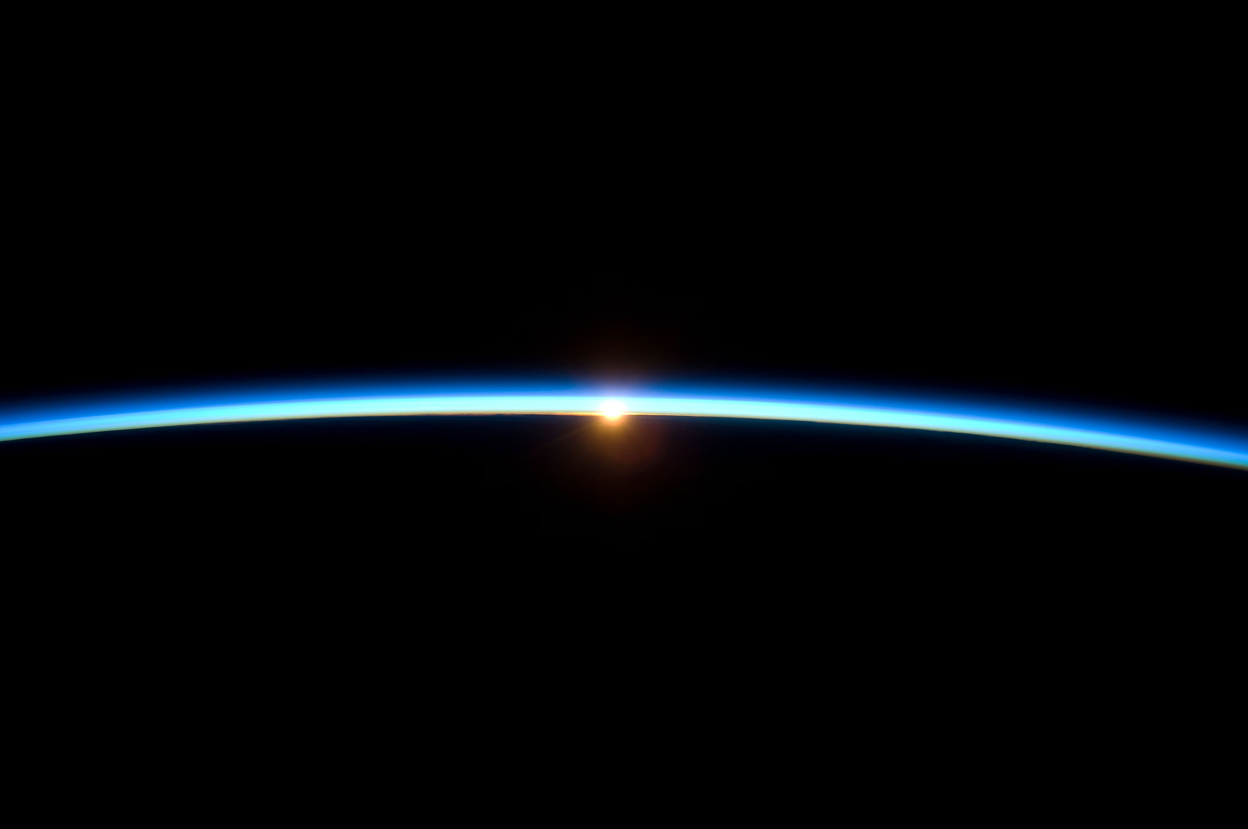
../_images/earth_thin_blue_line.avif — Fig. 5.1 Earth’s atmosphere as a thin blue line on the limb, photographed from the International Space Station during the STS-129 mission (November 2009). The atmosphere contains 99% of its mass below \(\sim\)30 km altitude (a mere 0.5% of Earth’s radius), yet this slender layer controls the surface temperature, shields life from harmful radiation, and mediates the exchange of volatiles between the interior and space. Credit: NASA/ISS Expedition 21 crew, public domain.#

5.1.1. Primary atmospheres#

Primary atmospheres are captured directly from the protoplanetary disk during planet formation. Because the disk is composed predominantly of hydrogen and helium (reflecting the solar composition), primary atmospheres are dominated by \(\mathrm{H_2}\) and He, with trace amounts of \(\mathrm{CH_4}\), \(\mathrm{NH_3}\), \(\mathrm{H_2O}\), and noble gases.

Only sufficiently massive bodies (those exceeding roughly \(5\)–\(10 \, \Mearth\)) can gravitationally capture and retain large quantities of nebular gas before the disk disperses (within \(\sim\)3–10 Myr; Lecture 2). The gas giants Jupiter and Saturn are the primary examples: their massive \(\mathrm{H_2}\)/He envelopes constitute the vast majority of their total mass, acquired during runaway gas accretion once the core mass reached a critical threshold (Fig. 5.2). The ice giants Uranus and Neptune also captured primary atmospheres, but far less gas: their envelopes are only \(\sim\)10–20% of their total mass, which reflects their slower growth and the disk’s dissipation.

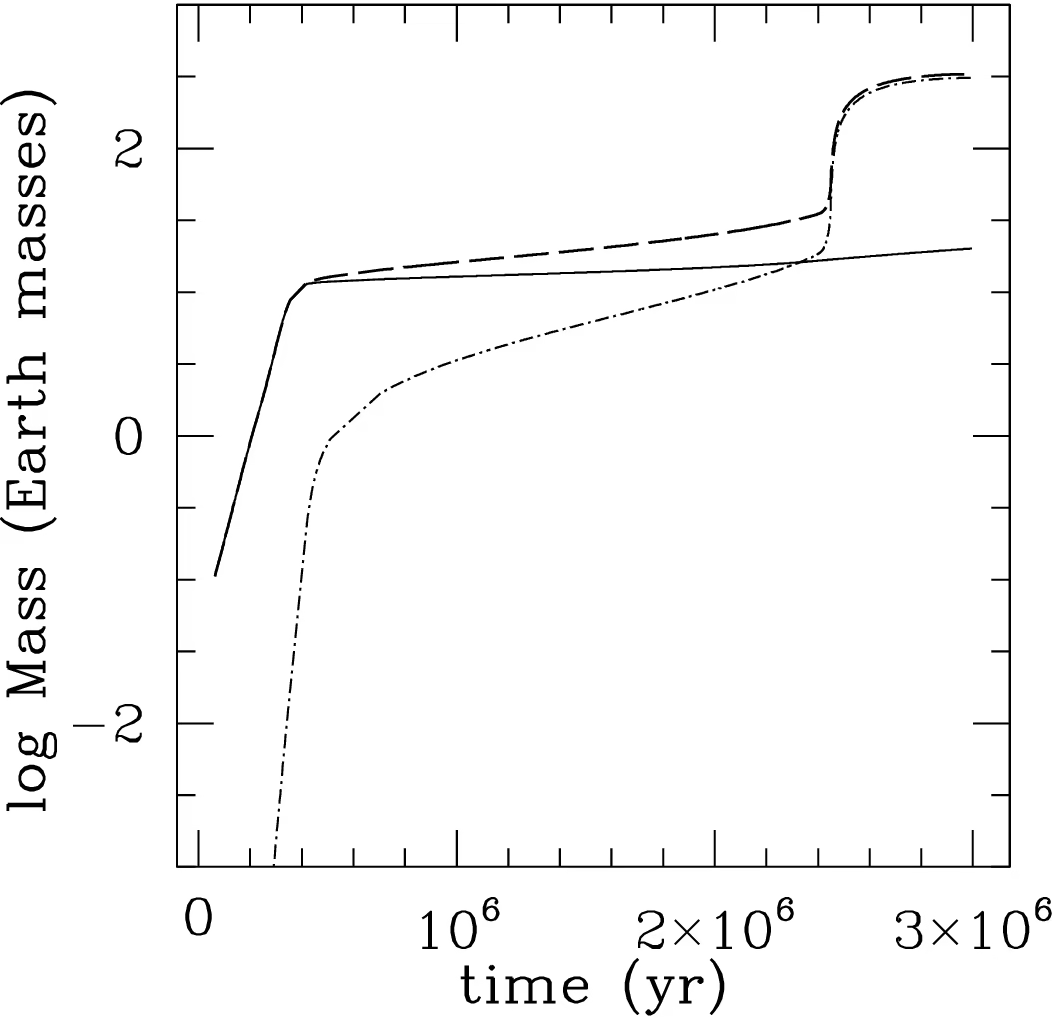
../_images/helled2014_core_accretion1.avif — Fig. 5.2 Growth of a giant planet by core accretion in the simulation of Jupiter’s formation at \(5.2\) AU introduced in Lecture 2: core mass (solid), envelope mass (dash-dotted) and total mass (dashed). The primary atmosphere is captured only in the last phase, after the envelope mass overtakes the core mass at \(2.3\) Myr and runaway gas accretion builds the \(\mathrm{H_2}\)/He envelope within the disk lifetime. Reproduced from Helled *et al.* [2014], Fig. 1; simulation from Lissauer *et al.* [2009].#

Terrestrial planets like Earth, Venus, and Mars were too small to capture much nebular gas. Any primordial hydrogen they did accrete was quickly lost to space (see atmospheric escape below). Their present-day atmospheres are therefore not primary.

5.1.2. Secondary atmospheres#

Secondary atmospheres are produced by outgassing: the release of volatiles from the planet’s interior through volcanism and magma ocean degassing. As discussed in Lecture 4, the speciation of outgassed volatiles depends on the oxygen fugacity of the magma (an effective partial pressure of \(\mathrm{O_2}\) that measures how oxidising or reducing the melt is): oxidising conditions produce \(\mathrm{CO_2}\), \(\mathrm{H_2O}\), and \(\mathrm{N_2}\), while reducing conditions produce \(\mathrm{H_2}\), CO, and \(\mathrm{N_2}\) (Fig. 5.3) [Hirschmann, 2012].

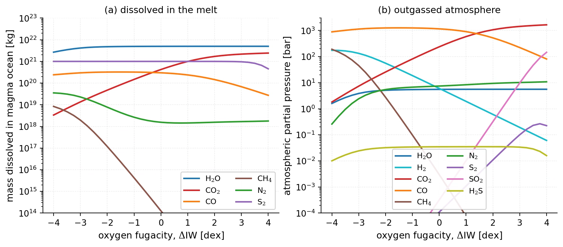
../_images/outgassing_speciation_fO21.avif — Fig. 5.3 Speciation of an outgassed atmosphere as a function of the melt oxygen fugacity, for Earth’s volatile inventory in equilibrium with a fully molten magma ocean at 2000 K (\(\Delta\)IW is the logarithmic shift from the iron-wüstite buffer; model of [Nicholls *et al.*, 2024], inventory of Krijt *et al.* [2023]). **(a)** Mass of each species dissolved in the melt: the water stays almost entirely in the magma. **(b)** Partial pressures in the atmosphere: carbon species dominate, as CO on the reduced side and \(\mathrm{CO_2}\) on the oxidised side, with \(\mathrm{H_2}\) and \(\mathrm{CH_4}\) under reducing conditions and \(\mathrm{SO_2}\) at the oxidised end. Course-original figure, discussed in Lecture 4.#

The present-day atmospheres of Venus (\(\mathrm{CO_2}\)-dominated) and Mars (\(\mathrm{CO_2}\)-dominated but much thinner) are essentially secondary atmospheres: their compositions reflect volcanic outgassing with relatively modest subsequent modification. Titan’s thick \(\mathrm{N_2}\) atmosphere also originated from outgassing (likely from the conversion of accreted \(\mathrm{NH_3}\)). Fig. 5.4 shows what a massive secondary atmosphere does to the surface beneath it.

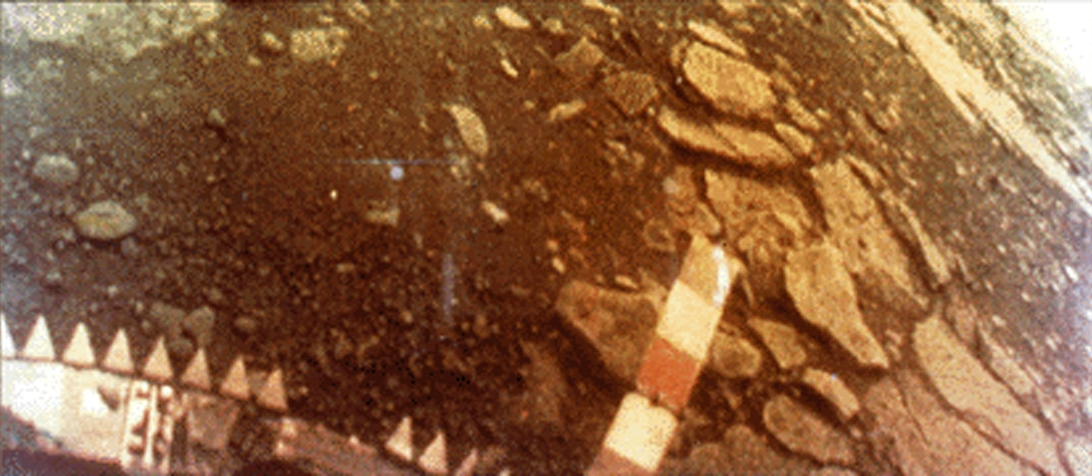
../_images/venera13_venus_surface.avif — Fig. 5.4 The surface of Venus photographed in colour by the Soviet *Venera 13* lander on 1 March 1982. The image shows flat basaltic rock slabs and soil lit by the orange light that filters through the thick \(\mathrm{CO_2}\) atmosphere (surface pressure 92 bar, temperature 737 K); the striped bar is a colour calibration target, and the toothed ring is part of the lander. The lander survived for 127 minutes before succumbing to the extreme conditions, a vivid demonstration of how a massive secondary atmosphere transforms a planet’s surface environment. Credit: USSR Academy of Sciences / NASA NSSDC, public domain.#

5.1.3. Tertiary atmospheres#

Tertiary atmospheres have been substantially modified from their outgassed composition by surface processes, photochemistry, or biology. Earth is the prime example: its original outgassed atmosphere was likely dominated by \(\mathrm{CO_2}\) and \(\mathrm{N_2}\) (similar to Venus), but billions of years of biological activity, particularly oxygenic photosynthesis, have transformed it into the \(\mathrm{N_2}\)/\(\mathrm{O_2}\) atmosphere we breathe today. Earth’s atmospheric \(\mathrm{O_2}\) (21% by volume) is entirely biogenic: it would disappear within a few million years if photosynthesis ceased [Catling and Kasting, 2017]. The build-up of this oxygen took most of Earth’s history (Fig. 5.5); Lecture 9 follows it in detail.

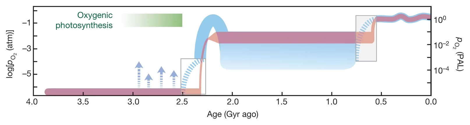
../_images/lyons2014_oxygen_history.avif — Fig. 5.5 Earth’s atmospheric oxygen through time, as \(p\mathrm{O_2}\) relative to the present atmospheric level (PAL, logarithmic scale). The atmosphere stayed anoxic (\(p\mathrm{O_2} < 10^{-5}\) PAL) for its first \(\sim\)2 Gyr, rose abruptly at the Great Oxidation Event (\(\sim\)2.4 Ga), held an intermediate plateau through the Proterozoic, and reached modern levels only in the Neoproterozoic and Phanerozoic. Reproduced from Lyons *et al.* [2014].#

5.1.4. Comparative atmospheric properties#

The diversity of atmospheres across the solar system is remarkable. The table below compares key properties for five representative bodies:

Property	Venus	Earth	Mars	Jupiter	Titan
Surface pressure (bar)	92	1.0	0.006	n/a	1.5
Surface temperature (K)	737	288	215	n/a	94
Dominant gas	\(\mathrm{CO_2}\) (96.5%)	\(\mathrm{N_2}\) (78%)	\(\mathrm{CO_2}\) (95%)	\(\mathrm{H_2}\) (90%)	\(\mathrm{N_2}\) (95%)
Secondary gas	\(\mathrm{N_2}\) (3.5%)	\(\mathrm{O_2}\) (21%)	\(\mathrm{N_2}\) (2.7%)	He (10%)	\(\mathrm{CH_4}\) (5%)
Mean molecular weight \(\mu\)	43.4	28.97	43.3	2.2	27.4
Atmosphere type	Secondary	Tertiary	Secondary	Primary	Secondary

Data from [de Pater and Lissauer, 2010] and [NASA Jet Propulsion Laboratory, 2026]. The fractional composition of these five atmospheres is shown in Fig. 5.6.

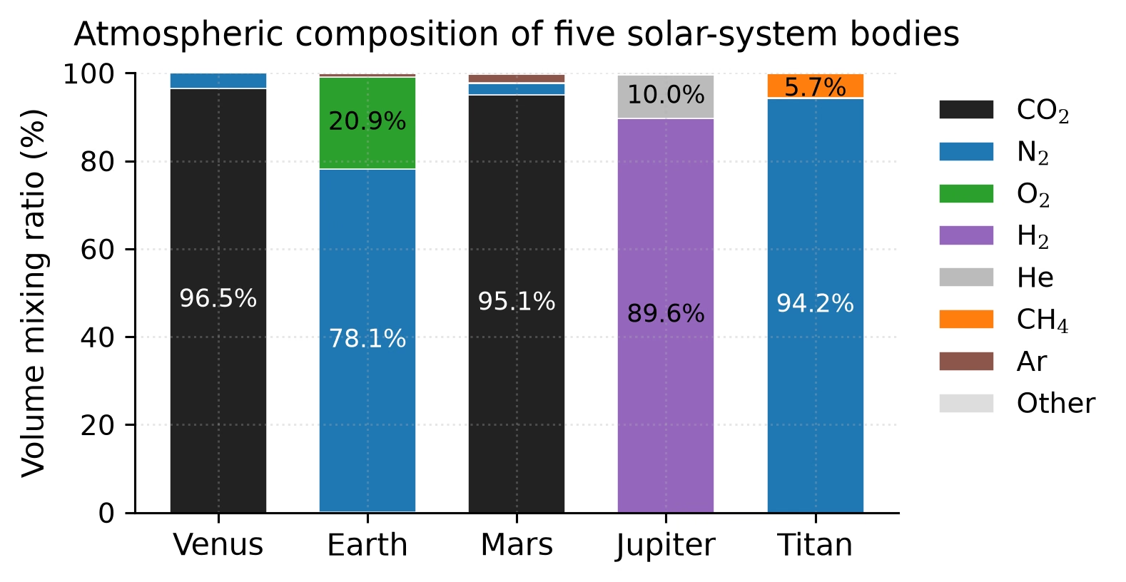
../_images/composition_bar.avif — Fig. 5.6 Atmospheric composition (by volume) for five representative solar system bodies. Venus and Mars are \(\mathrm{CO_2}\)-dominated secondary atmospheres; Earth’s \(\mathrm{N_2}\)/\(\mathrm{O_2}\) mix is biogenically modified (tertiary); Jupiter retains a primary \(\mathrm{H_2}\)/He envelope; Titan’s massive \(\mathrm{N_2}\) atmosphere is unusual for such a small body. Numbers rounded to one decimal place. Data from [NASA Jet Propulsion Laboratory, 2026]. Course-original figure.#

5.2. Hydrostatic equilibrium#

The vertical structure of any atmosphere is governed by the balance between gravity pulling gas downward and the pressure gradient pushing it upward. This balance, called hydrostatic equilibrium, is the most fundamental equation of atmospheric physics.

5.2.1. Derivation#

Consider a thin horizontal slab of atmosphere with cross-sectional area \(A\), thickness \(\dd z\), and density \(\rho(z)\) at height \(z\) above the surface. The forces on this slab are:

Pressure from below (pushing up): \(P(z) \cdot A\)
Pressure from above (pushing down): \(P(z + \dd z) \cdot A\)
Weight (pulling down): \(\rho(z) \, g \, A \, \dd z\)

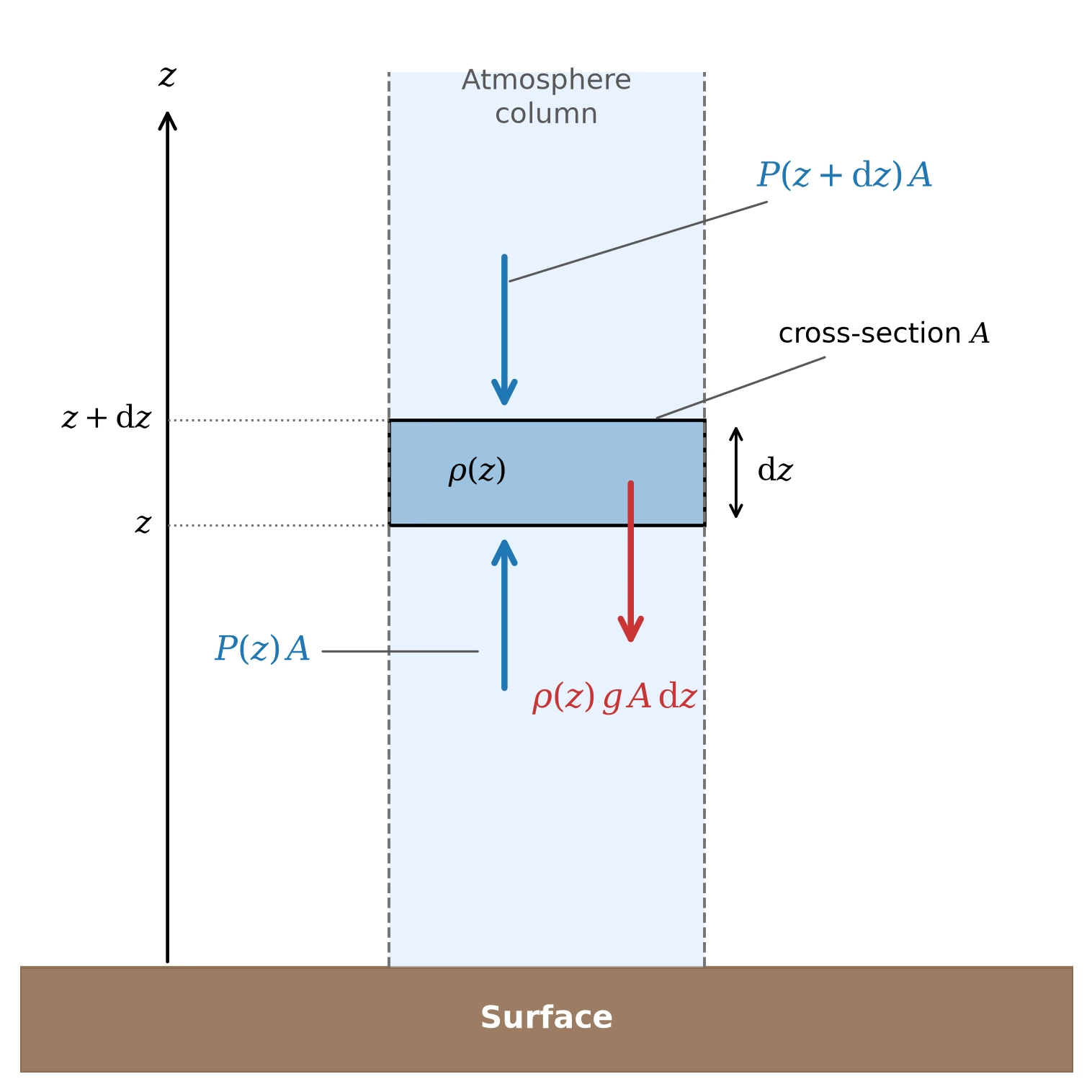
../_images/hydrostatic_slab.avif — Fig. 5.7 Force balance on a thin horizontal slab of atmosphere with cross-sectional area \(A\), thickness \(\dd z\), and density \(\rho(z)\). Pressure acting on the lower face pushes the slab up with force \(P(z)\,A\) (blue), while pressure on the upper face pushes down with force \(P(z+\dd z)\,A\) (blue) and gravity pulls the slab down with its weight \(\rho(z)\,g\,A\,\dd z\) (red). Setting the net force to zero and taking the limit \(\dd z \to 0\) yields the equation of hydrostatic equilibrium. Course-original figure.#

In equilibrium (Fig. 5.7), the net upward pressure force balances the weight:

\[ P(z) \, A - P(z + \dd z) \, A = \rho(z) \, g \, A \, \dd z \]

Dividing by \(A \, \dd z\) and taking the limit \(\dd z \to 0\), in which \([P(z + \dd z) - P(z)]/\dd z\) becomes the derivative \(\dv{P}{z}\):

(5.1)#\[ \dv{P}{z} = -\rho \, g \]

This is the equation of hydrostatic equilibrium. The pressure decreases with altitude because each layer must support the weight of everything above it. The minus sign reflects that pressure decreases as height increases.

5.2.2. The ideal gas law in atmospheric form#

To solve Eq. (5.1), we need a relation between pressure and density. For an atmosphere behaving as an ideal gas:

(5.2)#\[ P = n \kB T = \frac{\rho \kB T}{\mu \, m_u} \]

where \(n\) is the number density, \(\kB = 1.381 \times 10^{-23}\) J K\(^{-1}\) is the Boltzmann constant, \(T\) is the temperature, \(\mu\) is the mean molecular weight (in atomic mass units), and \(m_u = 1.661 \times 10^{-27}\) kg is the atomic mass unit.

Fig. 5.8 shows what this form of the ideal gas law implies: at fixed temperature the density is proportional to the pressure, and at fixed pressure a heavier or a colder gas is denser.

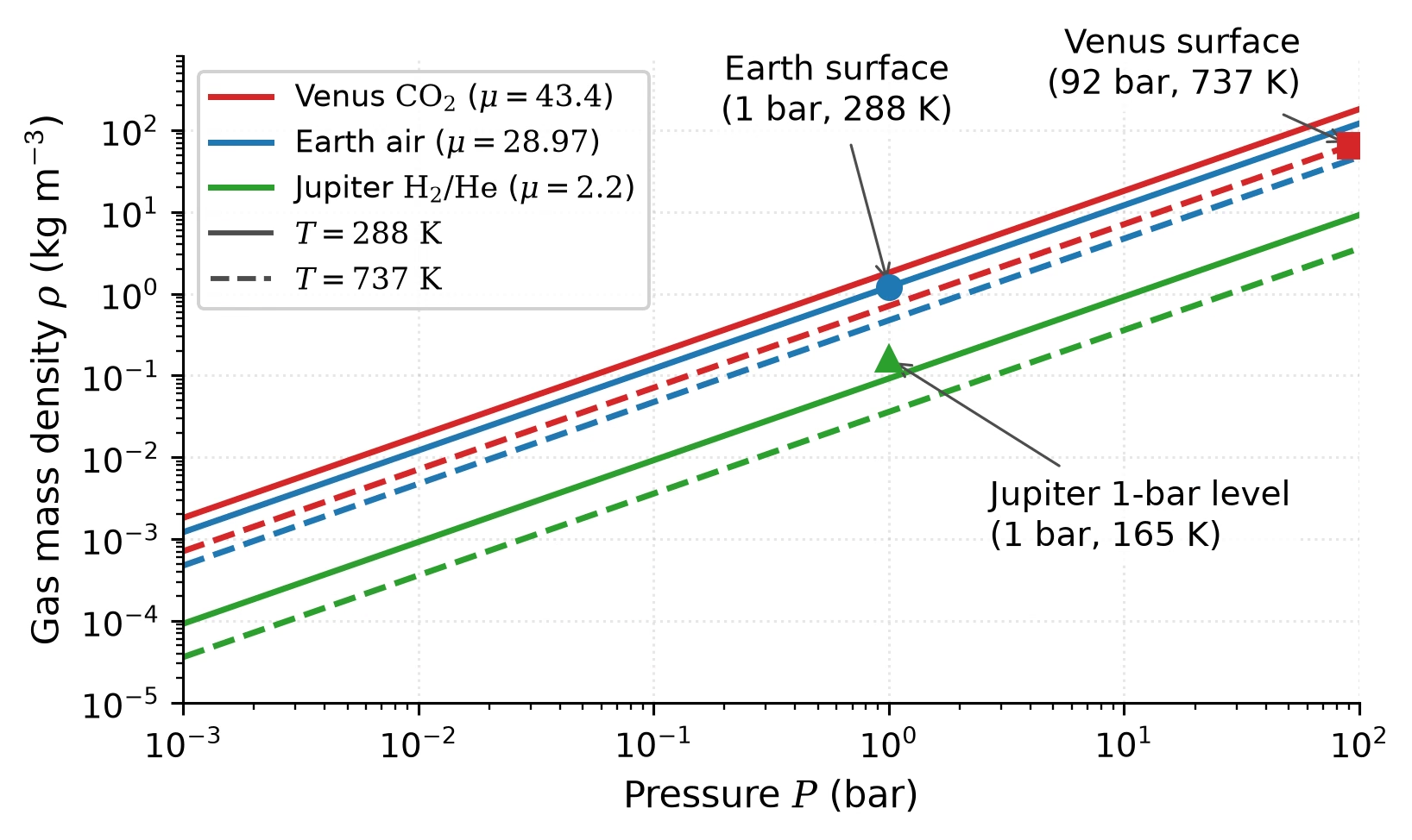
../_images/ideal_gas_density.avif — Fig. 5.8 Gas mass density \(\rho = P \mu m_u/(\kB T)\) as a function of pressure for three mean molecular weights, \(\mu = 2.2\) (H\(_2\)/He, Jupiter), \(28.97\) (Earth air) and \(43.4\) (CO\(_2\), Venus), at \(T = 288\) K (solid) and \(T = 737\) K (dashed). The markers give the Earth surface (1 bar, 288 K), the Venus surface (92 bar, 737 K) and the 1 bar level of Jupiter (165 K). At fixed \(T\) the lines are parallel in the log-log plane, so the density at a given pressure is set by \(\mu\); heating from 288 K to 737 K lowers the density by the ratio of the two temperatures. Course-original figure.#

5.2.3. The barometric formula#

If we assume the atmosphere is isothermal (constant \(T\)) and that \(g\) is constant (valid for the lower atmosphere where \(z \ll R_{\text{planet}}\)), we can substitute the ideal gas law into the hydrostatic equation. From Eq. (5.2), \(\rho = P \mu m_u / (\kB T)\), so:

\[ \dv{P}{z} = -\frac{P \mu \, m_u \, g}{\kB T} \]

This is a separable first-order ODE. Integrating from the surface (\(z = 0\), \(P = P_0\)) to height \(z\):

(5.3)#\[ P(z) = P_0 \exp\!\left(-\frac{z}{H}\right) \]

where we have defined the pressure scale height \(H\):

(5.4)#\[ H = \frac{\kB T}{\mu \, m_u \, g} \]

The barometric formula tells us that atmospheric pressure decreases exponentially with altitude. Every scale height \(H\), the pressure drops by a factor of \(e \approx 2.718\). This exponential decay is why atmospheres are thin compared to the size of the planet: for an isothermal column, 99% of the mass lies below \(4.6\,H\); in the real atmosphere, colder layers aloft compress this to \(\sim\)30 km for Earth.

Integrating the hydrostatic equation over the whole column instead gives the surface pressure as the weight of the atmosphere per unit area, \(P_0 = m_{\mathrm{col}}\, g\), where \(m_{\mathrm{col}} = \int_0^\infty \rho \, dz\) is the column mass. For Earth, \(m_{\mathrm{col}} = P_0/g \approx 1.03 \times 10^4\) kg m\(^{-2}\), about ten tonnes above every square metre.

Fig. 5.9 plots the same exponential profile on a linear and on a logarithmic pressure axis.

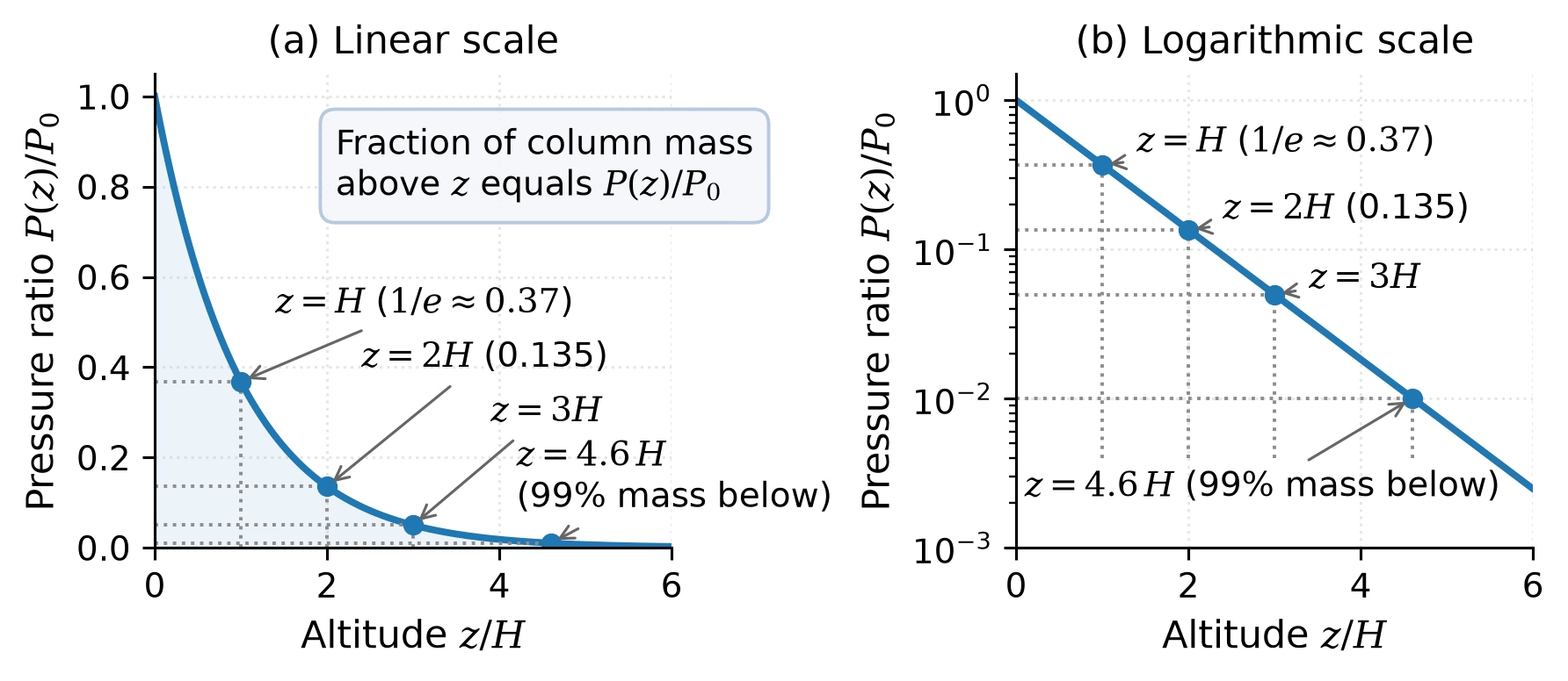
Fig. 5.9 The barometric formula \(P(z)/P_0 = e^{-z/H}\) on (a) a linear and (b) a logarithmic pressure axis. The marked levels are \(z = H\) (\(P/P_0 = 1/e \approx 0.37\)), \(z = 2H\) (\(0.135\)), \(z = 3H\) (\(0.050\)) and \(z = 4.6\,H\) (\(0.010\)), the level below which 99% of the column mass sits in an isothermal atmosphere. Because hydrostatic balance makes \(P(z)\) equal to the weight of the overlying column, the pressure ratio at any level is also the fraction of the column mass above it. On the logarithmic axis the profile is a straight line: every scale height lowers \(\ln(P/P_0)\) by one. Course-original figure.#

5.3. Blackboard derivation: The atmospheric scale height#

Blackboard derivation: Atmospheric scale height from hydrostatic equilibrium

Goal: Derive the atmospheric scale height \(H = \kB T / (\mu \, m_u \, g)\) from hydrostatic equilibrium combined with the ideal gas law, and compute \(H\) for Earth, Mars, Venus, Jupiter, and Titan.

Setup.

We start from the equation of hydrostatic equilibrium (Eq. (5.1)) and the ideal gas law (Eq. (5.2)):

\[ \dv{P}{z} = -\rho \, g \qquad \text{and} \qquad P = \frac{\rho \kB T}{\mu \, m_u} \]

Our goal is to find the characteristic length scale over which pressure varies: the scale height.

Fig. 5.10 shows the slab that the force balance is written for.

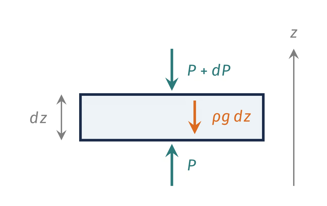
../_images/board_sketch_l05.avif — Fig. 5.10 Setup sketch of the board derivation of the scale height: a thin horizontal slab of thickness \(dz\) at altitude \(z\), pushed up by the pressure \(P\) from below, pushed down by \(P + dP\) from above, and pulled down by its weight \(\rho g\,dz\) per unit area. Course-original figure.#

Derivation.

Rearranging the ideal gas law to express \(\rho\) in terms of \(P\):

\[ \rho = \frac{P \, \mu \, m_u}{\kB T} \]

Substituting into the hydrostatic equation:

\[ \dv{P}{z} = -\frac{\mu \, m_u \, g}{\kB T} \, P \]

This has the form \(\dv{P}{z} = -P/H\), where:

(5.5)#\[ \boxed{H = \frac{\kB T}{\mu \, m_u \, g}} \]

The scale height has a clear physical interpretation:

Higher temperature \(T\) → larger \(H\): hotter gas has more thermal energy, so it extends further against gravity.
Heavier molecules (larger \(\mu\)) → smaller \(H\): heavier molecules are harder to loft.
Stronger gravity \(g\) → smaller \(H\): stronger gravity compresses the atmosphere more.

Application: scale heights across the solar system.

We can now compute scale heights for several bodies using their characteristic atmospheric temperatures, compositions, and surface gravities:

Body	\(T\) (K)	\(\mu\)	\(g\) (m s\(^{-2}\))	\(H\) (km)
Venus	737	43.4	8.87	15.9
Earth	288	28.97	9.81	8.4
Mars	215	43.3	3.72	11.1
Jupiter	165	2.2	24.8	25
Titan	94	27.4	1.35	21

Worked example for Earth:

\[ H_\oplus = \frac{1.381 \times 10^{-23} \times 288}{28.97 \times 1.661 \times 10^{-27} \times 9.81} = \frac{3.98 \times 10^{-21}}{4.72 \times 10^{-25}} \approx 8400 \text{ m} \approx 8.4 \text{ km} \]

This matches our everyday experience: commercial aircraft cruise at \(\sim\)10–12 km altitude, where the pressure is roughly \(0.2\)–\(0.3\) atm (about 1.2–1.4 scale heights up).

Note: Jupiter’s scale height is large despite its strong gravity because \(\mathrm{H_2}\) has a very low molecular weight (\(\mu = 2.2\)). Titan’s scale height is large because its gravity is weak (\(g = 1.35\) m s\(^{-2}\)): Titan’s atmosphere extends to a proportionally much greater height than Earth’s, despite being colder.

Fig. 5.11 recomputes \(H\) from the entries of the table above and sorts the five bodies by the result.

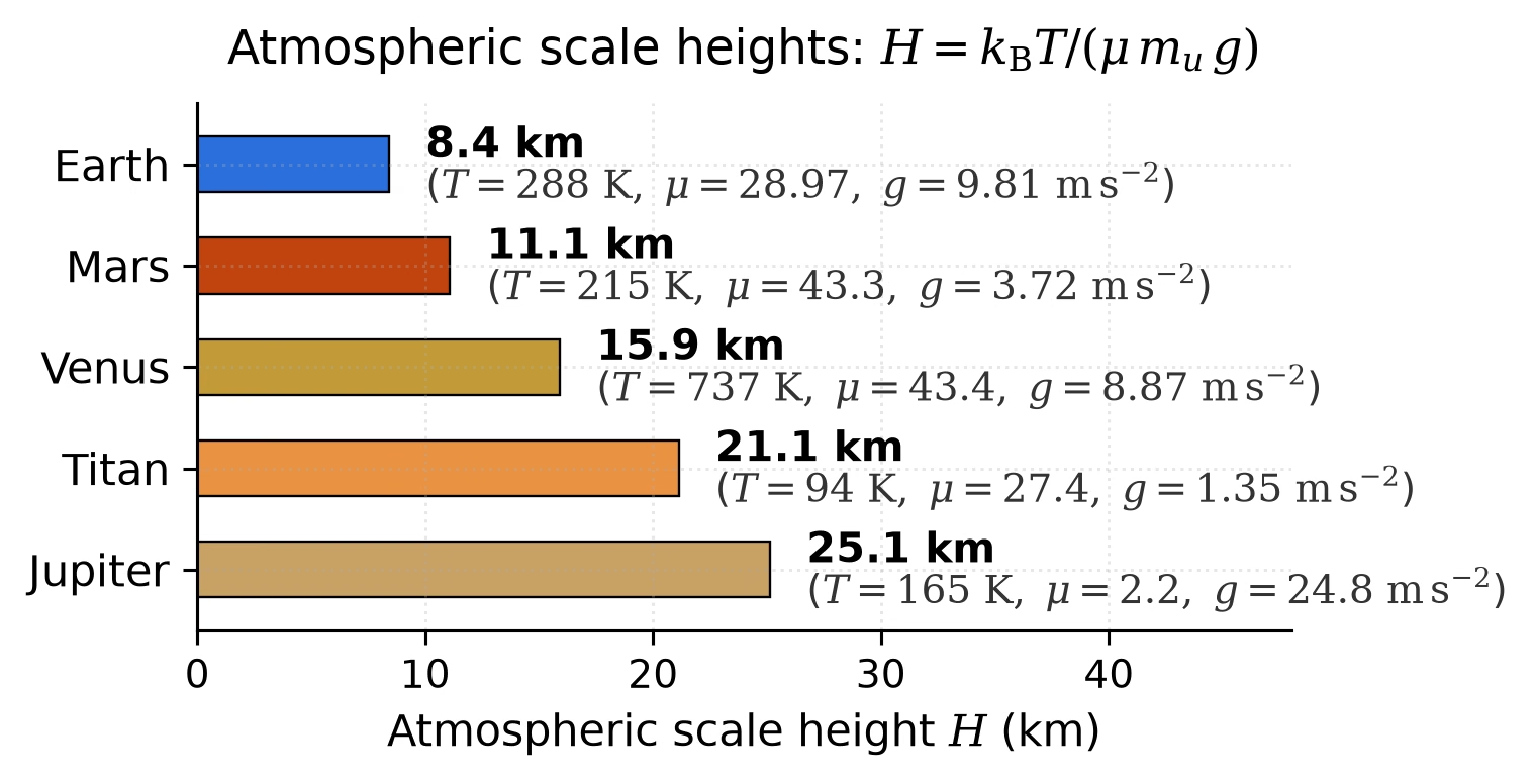
../_images/scale_height_bar.avif — Fig. 5.11 Atmospheric scale heights \(H = \kB T/(\mu m_u g)\) for Venus, Earth, Mars, Jupiter and Titan, computed from the temperature, mean molecular weight and surface gravity listed in the table above and sorted by \(H\). Jupiter, with the lightest gas, and Titan, with the weakest gravity, have the largest scale heights although both are cold; Earth, warm but with a strong gravity and a moderately heavy gas, has the smallest. All three parameters matter. Course-original figure.#

5.4. Vertical structure#

Real atmospheres are not isothermal: temperature varies with altitude, creating distinct layers characterised by different physical processes. These layers are defined by the sign of the temperature gradient \(\dv{T}{z}\).

5.4.1. Troposphere#

The troposphere is the lowest layer, heated primarily from below by the surface (which absorbs sunlight and re-emits thermal radiation). Warm air near the surface rises, cool air aloft sinks: this is convection, the same process we encountered in planetary interiors (Lecture 3). Convection keeps the troposphere well-mixed and imposes a characteristic temperature decrease with altitude called the lapse rate.

For a parcel of dry air rising adiabatically (without exchanging heat with its surroundings), the temperature decreases at the dry adiabatic lapse rate:

(5.6)#\[ \Gamma_d = -\dv{T}{z} = \frac{g}{c_p} \]

where \(c_p\) is the specific heat capacity at constant pressure. For Earth, \(g = 9.81\) m s\(^{-2}\) and \(c_p \approx 1004\) J kg\(^{-1}\) K\(^{-1}\) (for dry air), giving \(\Gamma_d \approx 9.8\) K km\(^{-1}\). The observed average lapse rate (\(\sim 6.5\) K km\(^{-1}\)) is lower because of latent heat released by condensing water vapour, which warms a rising parcel relative to a dry one and so reduces the cooling rate. The lapse rate of a saturated parcel undergoing reversible condensation is the moist adiabatic lapse rate (Fig. 5.12).

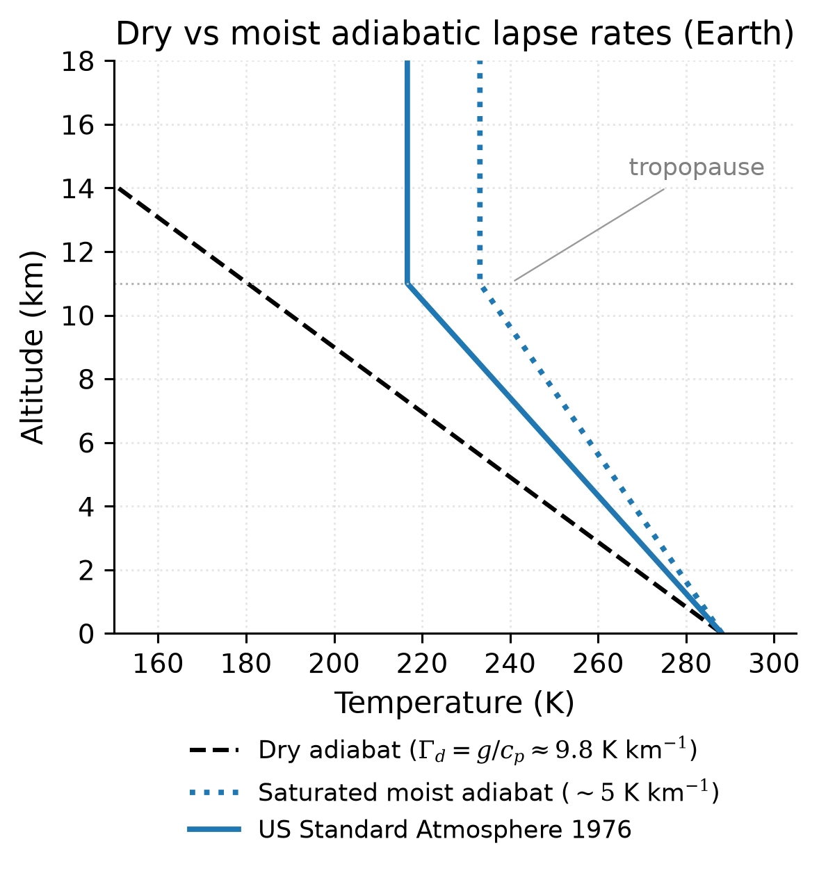
../_images/dry_moist_adiabat.avif — Fig. 5.12 Dry adiabatic lapse rate (\(\Gamma_d = g/c_p \approx 9.8\) K km\(^{-1}\), dashed) compared with a representative saturated moist adiabat (\(\sim 5\) K km\(^{-1}\) in the warm lower troposphere, dotted) and the US Standard Atmosphere 1976 reference profile (solid), a defined standard for year-round midlatitude conditions [NOAA and NASA and U.S. Air Force, 1976]. The moist adiabat is shallower than the dry adiabat because condensing water vapour releases latent heat to the rising parcel; the reference profile’s tropospheric lapse rate (6.5 K km\(^{-1}\), close to the observed midlatitude mean) lies between the two limits. Above the tropopause the adiabats no longer apply: the profile becomes nearly isothermal, and the stratospheric warming begins above the 18 km top of this plot. Course-original figure.#

Earth’s troposphere extends from the surface to the tropopause at \(\sim\)12 km altitude (varying from \(\sim\)8 km at the poles to \(\sim\)17 km at the equator).

5.4.2. Stratosphere#

Above the tropopause, temperature increases with altitude in the stratosphere. On Earth, this temperature inversion is caused by the absorption of solar ultraviolet radiation by the ozone layer (\(\mathrm{O_3}\)), centred at \(\sim\)25 km altitude. The heating by UV absorption creates a stable, non-convective layer: air parcels displaced upward find themselves cooler and denser than their surroundings and sink back down.

Earth’s stratosphere extends to the stratopause at \(\sim\)50 km. Stratospheric inversions can also be driven by organic aerosol absorption rather than ozone, as seen in the detached photochemical haze layers of Titan (Fig. 5.13).

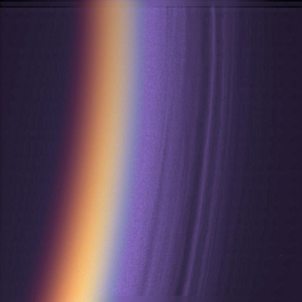
../_images/titan_haze_pia06160.avif — Fig. 5.13 Detached haze layers in Titan’s upper atmosphere imaged at the limb by the Cassini ISS narrow-angle camera (PIA06160). Multiple distinct layers from \(\sim\)200 km up to \(\sim\)500 km altitude are produced by photochemistry of \(\mathrm{CH_4}\) in the stratosphere, generating the organic aerosols that give Titan its orange colour and heat the stratosphere by absorbing UV. Credit: NASA/JPL/Space Science Institute, public domain.#

5.4.3. Mesosphere and thermosphere#

Above the stratopause, the mesosphere (50–85 km) cools with altitude again as ozone heating diminishes. The mesopause at \(\sim\)85 km is the coldest point in Earth’s atmosphere (\(\sim\)190 K).

Above this, the thermosphere (85–600 km) is heated by the absorption of extreme ultraviolet (EUV) radiation and energetic particles, with temperatures rising steeply to \(>\)1000 K. The thermosphere merges into the exosphere, the outermost region where the mean free path, the average distance a molecule travels between two collisions, exceeds the scale height and molecules on ballistic trajectories can escape to space (Fig. 5.14); the exobase in Atmospheric escape makes this boundary precise.

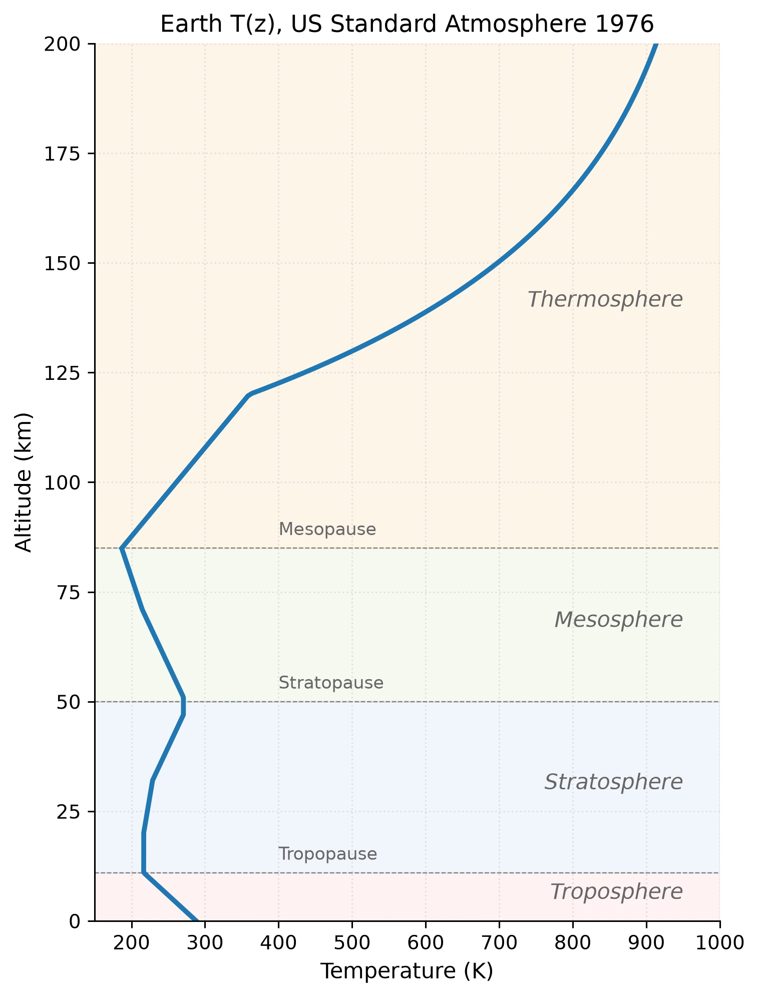
../_images/earth_tz_layers.avif — Fig. 5.14 Earth’s vertical temperature profile from the US Standard Atmosphere 1976, with the four named layers (troposphere, stratosphere, mesosphere, thermosphere) shaded. Pause levels (tropopause \(\sim\)11 km, stratopause \(\sim\)50 km, mesopause \(\sim\)85 km) are marked with dashed grey lines. The sign of \(\dv{T}{z}\) flips at each pause, which reflects the transition between dominant heating sources (surface re-radiation in the troposphere, ozone UV absorption in the stratosphere, EUV absorption in the thermosphere). Data: US Standard Atmosphere 1976 [NOAA and NASA and U.S. Air Force, 1976]. Course-original figure.#

5.4.4. Comparative vertical structures#

The vertical structure varies dramatically across the solar system [Catling and Kasting, 2017]:

Venus: A massive troposphere extends to \(\sim\)65 km. Above the cloud deck (\(\sim\)48–70 km), temperature decreases slowly. There is no Earth-like stratospheric temperature inversion because Venus lacks an ozone layer.
Mars: A thin troposphere (\(\sim\)40 km) directly overlain by a thermosphere. Mars also lacks an appreciable ozone layer and stratospheric inversion.
Jupiter: The troposphere extends deep into the planet (hundreds of kilometres). The stratosphere is heated by \(\mathrm{CH_4}\) and hydrocarbon haze absorption. There is no solid surface; pressure increases continuously with depth.
Titan: A thick troposphere (\(\sim\)40 km), a stratosphere extending up to \(\sim\)300 km heated by organic haze absorption, and an extended thermosphere reaching \(\sim\)1400 km, remarkably high for such a small body, which reflects Titan’s weak gravity and large scale height. The Huygens-derived T(z) profile is shown in Fig. 5.15; the canonical Venus T(z) used for comparison is shown in Fig. 5.16.

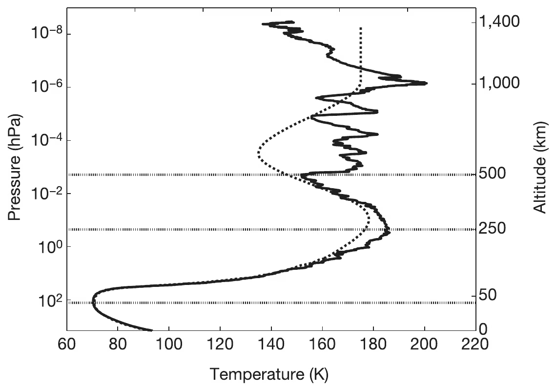
../_images/fulchignoni2005_titan_tz.avif — Fig. 5.15 Titan’s atmospheric temperature profile from the *Huygens* Atmospheric Structure Instrument (HASI) descent on 14 January 2005. Solid line: HASI measurements; dashed line: pre-encounter Titan engineering model. Above 160 km, \(T\) and \(P\) are derived from the measured density via the ideal gas law; below 160 km, \(T\) is measured directly by the TEM sensor. Horizontal markers indicate the mesopause (152 K at 490 km), stratopause (186 K at 250 km), and tropopause (70.43 K at 44 km). Wave-like fluctuations above 250 km reflect gravity-wave activity; Titan’s methane clouds and methane cycle are explored in Lecture 6 and Lecture 11. Reproduced from [Fulchignoni *et al.*, 2005], Fig. 2.#

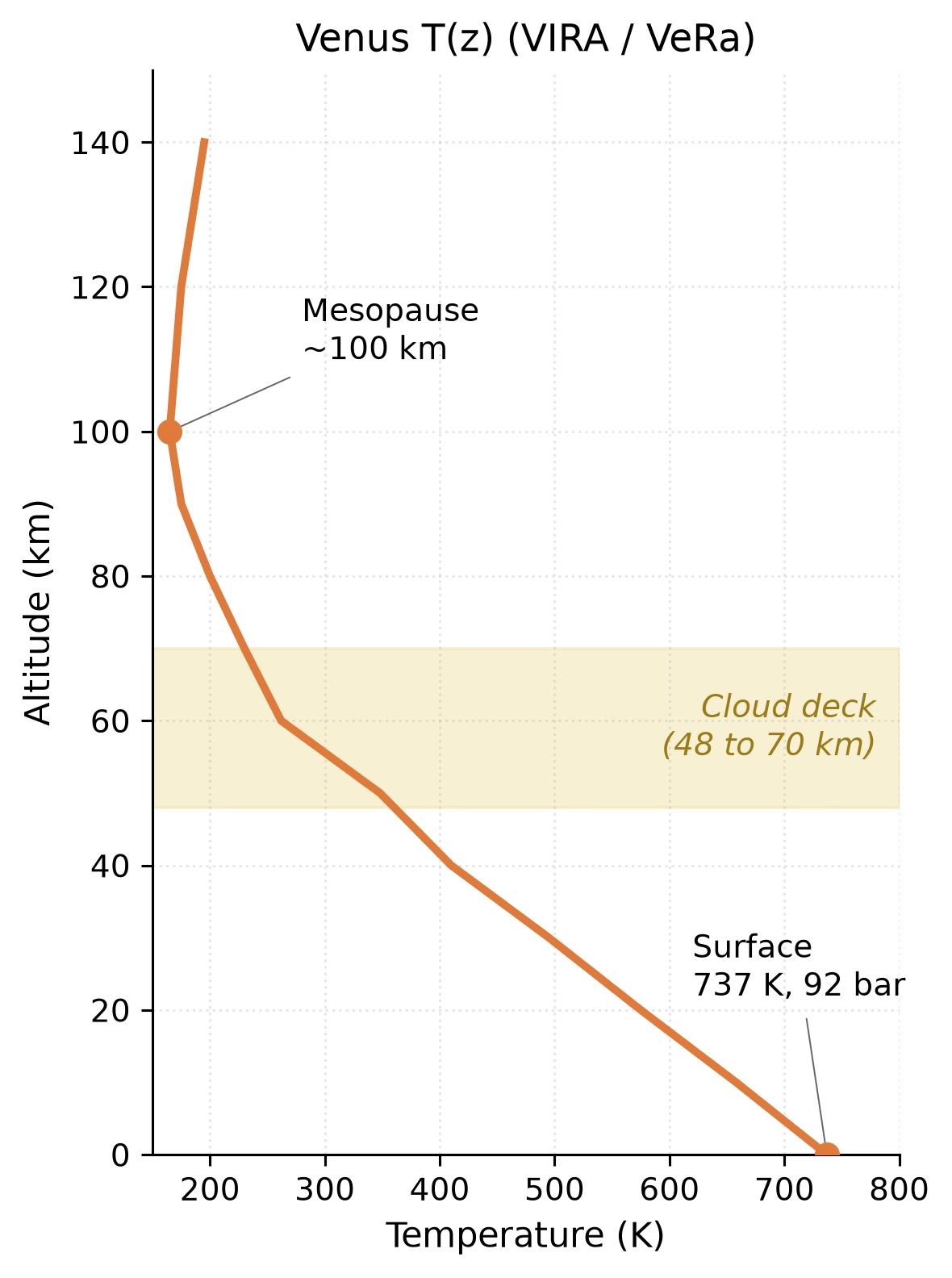
../_images/venus_tz_vira.avif — Fig. 5.16 Venus T(z) profile combining Pioneer Venus / VIRA [Seiff *et al.*, 1985] lower-atmosphere data with VeRa (Venus Express) radio-occultation results [Tellmann *et al.*, 2009]. The profile falls monotonically from the 737 K, 92 bar surface through the cloud deck (48 to 70 km, shaded) to the mesopause near 100 km, with no ozone-driven stratospheric inversion. The near-adiabatic deep troposphere reflects efficient convection in a \(\mathrm{CO_2}\)-dominated, optically thick atmosphere. Pedagogical fit; not a direct reproduction. Course-original figure.#

A striking unifying observation is that, despite differences of orders of magnitude in surface gravity, composition, and stellar irradiation, the tropopause occurs at a pressure near \(0.1\) bar in nearly every thick atmosphere of the solar system (Fig. 5.17). Robinson and Catling [2014] showed that this is a consequence of pressure-dependent infrared transparency: at lower pressures the atmosphere becomes optically thin to thermal radiation, convection ceases, and any UV/shortwave absorber aloft creates a stratospheric inversion; the combination freezes in a near-universal temperature minimum near 0.1 bar.

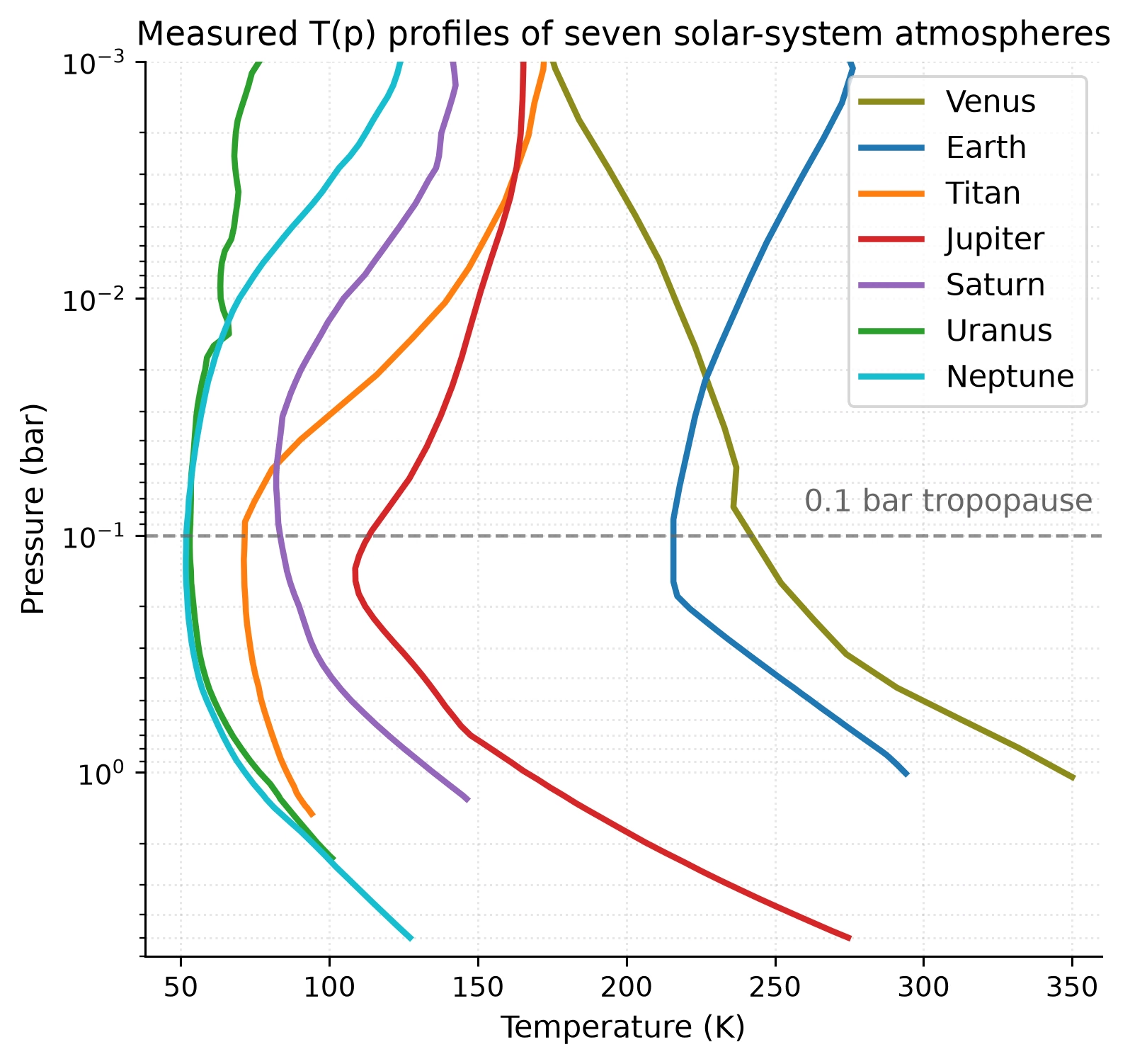
../_images/atmosphere_tp_robinson.avif — Fig. 5.17 Measured vertical temperature profiles of seven solar system atmospheres (Venus, Earth, Titan, Jupiter, Saturn, Uranus, Neptune) plotted against pressure (note the log scale, with low pressures at the top). The tropopause consistently occurs near 0.1 bar in Earth, Titan, and the four giant planets; Venus, which lacks a strong stratospheric inversion, shows only a weak global-mean minimum there [Robinson and Catling, 2014]. Profiles digitized from Robinson and Catling [2014], Fig. 1, and replotted; the underlying data come from spacecraft radio occultations, infrared spectroscopy, and reference atmosphere compilations.#

5.5. Radiative transfer basics#

While convection dominates energy transport in the troposphere, radiation is the primary mechanism by which energy enters and leaves the atmosphere. Understanding how radiation interacts with atmospheric gases is essential for explaining why planets have the temperatures they do.

5.5.1. Absorption, emission, and scattering#

When a beam of radiation passes through an atmosphere, three things can happen:

Absorption: A gas molecule absorbs a photon, converting radiative energy into internal energy (vibrational, rotational, or electronic excitation). The key atmospheric absorbers are greenhouse gases: \(\mathrm{CO_2}\), \(\mathrm{H_2O}\), \(\mathrm{CH_4}\), \(\mathrm{O_3}\), and \(\mathrm{N_2O}\). These molecules have vibrational and rotational modes that absorb strongly in the infrared, precisely the wavelengths at which warm planetary surfaces emit.
Emission: By Kirchhoff’s law, any gas that absorbs radiation at a given wavelength also emits at that wavelength when it is warm. This thermal emission is the mechanism by which the atmosphere radiates energy to space.
Scattering: Photons are redirected without being absorbed. Rayleigh scattering by \(\mathrm{N_2}\) and \(\mathrm{O_2}\) (which goes as \(\lambda^{-4}\)) explains why the sky is blue and sunsets are red (Fig. 5.18). Mie scattering by larger particles (aerosols, cloud droplets) is less wavelength-dependent.

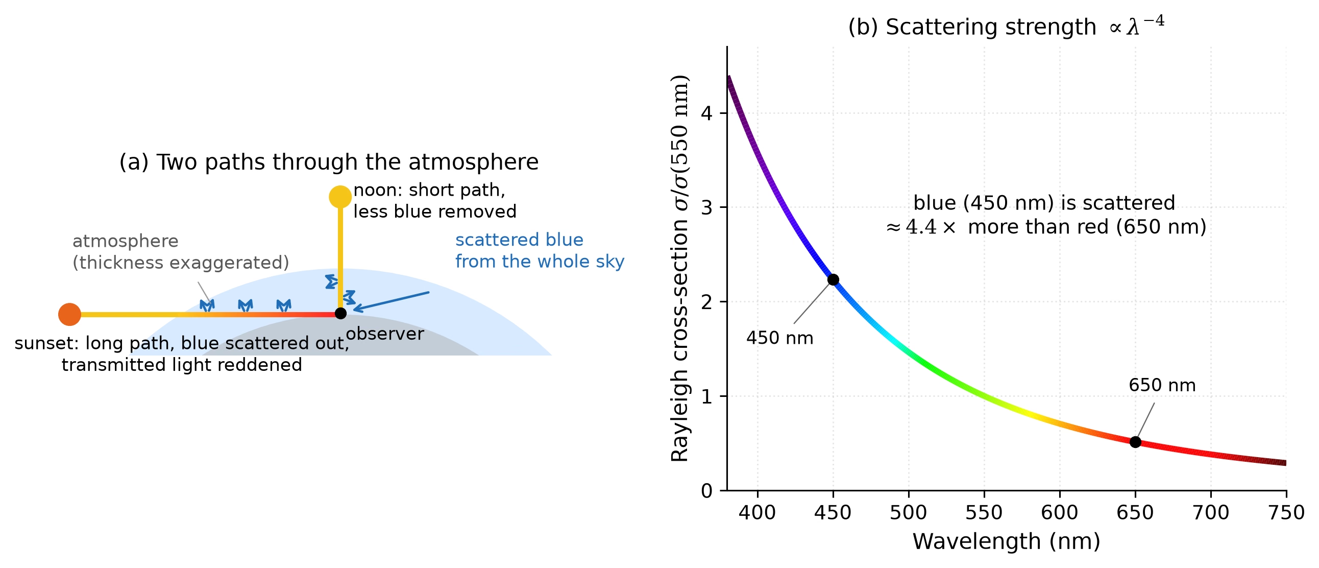
../_images/rayleigh_scattering.avif — Fig. 5.18 Rayleigh scattering and the colour of the sky. Panel (a): two sunlight paths to the same observer, with the atmosphere thickness exaggerated for clarity. At noon the beam crosses the atmosphere nearly vertically and loses much less blue light to scattering than at sunset; the scattered blue reaches the eye from every direction, so the sky looks blue. At sunset the beam follows a slant path roughly 40 times longer (the tangent-path estimate \(\sqrt{2R/H} \approx 40\) for a scale height of \(H \approx 8.5\) km), so most of the blue is scattered out before arrival and the transmitted light is reddened. Panel (b): relative Rayleigh scattering cross-section \(\sigma \propto \lambda^{-4}\) across the visible band, normalised to 550 nm; blue light (450 nm) is scattered about 4.4 times more strongly than red light (650 nm). Course-original figure.#

The wavelength dependence of stellar versus planetary emission is the physical basis of the greenhouse effect (Fig. 5.19): the Sun radiates predominantly in the visible while a \(\sim 300\) K planet radiates in the thermal infrared, and atmospheric gases can be opaque at one set of wavelengths while transparent at the other.

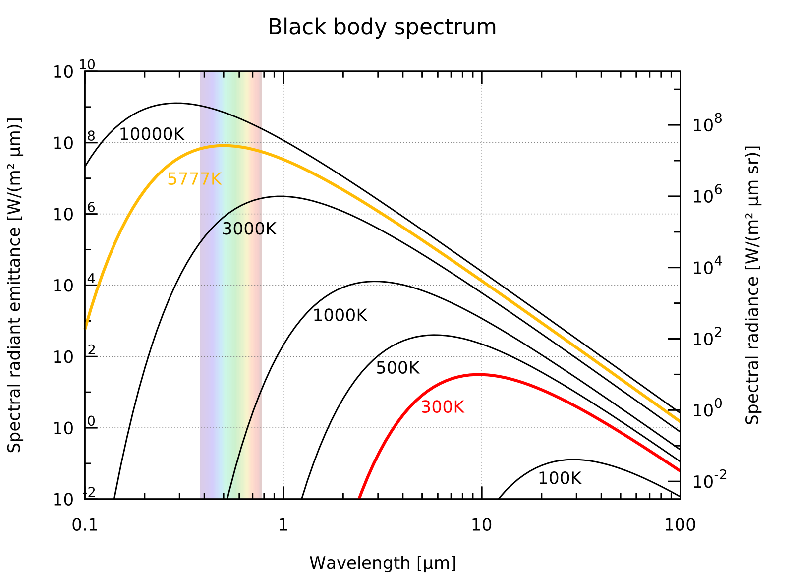
../_images/blackbody_spectrum.svg — Fig. 5.19 Blackbody radiation curves for objects at several temperatures (representative of stellar and planetary emission). The Sun (\(\sim\)5800 K) emits primarily at visible wavelengths (\(\sim\)0.5 \(\mu\)m), while a planet at \(\sim\)300 K emits in the thermal infrared (\(\sim\)10 \(\mu\)m). Credit: Wikimedia Commons, public domain.#

5.5.2. Optical depth#

The cumulative effect of absorption along a path through the atmosphere is quantified by the optical depth \(\tau\):

(5.7)#\[ \tau = \int_0^s \kappa \, \rho \, \dd s' \]

where \(\kappa\) is the mass absorption coefficient (m\(^2\) kg\(^{-1}\)), \(\rho\) is the gas density, and \(s\) is the path length. Alternatively, using the number density \(n\) and the absorption cross-section \(\sigma\): \(\tau = \int n \sigma \, \dd s'\).

The optical depth is dimensionless. It counts how many absorption lengths the radiation crosses, where one absorption length is the distance over which the intensity falls by a factor \(e\) (the Beer-Lambert law in the next section). The geometric length of one unit of \(\tau\) is \(1/(n\sigma)\), the mean free path of a photon: short in a dense layer, long in a thin one. So \(\tau\) measures how much absorption a path contains, not how long the path is:

\(\tau \ll 1\): Optically thin, most radiation passes through without being absorbed.
\(\tau \gg 1\): Optically thick, radiation is strongly absorbed; only photons emitted near the “top” of the absorbing layer escape.

5.5.3. Beer-Lambert law#

For a beam of radiation with initial intensity \(I_0\) passing through a medium of optical depth \(\tau\):

(5.8)#\[ I = I_0 \, e^{-\tau} \]

This exponential attenuation law, the Beer-Lambert law, shows that intensity decreases by a factor of \(e\) for each unit of optical depth traversed.

5.5.4. The atmospheric photosphere concept#

Just as a star has a photosphere, the layer from which photons escape to space, a planet’s atmosphere has an effective emission level at approximately \(\tau \approx 1\) (when looking from space downward at infrared wavelengths). Photons emitted from below this level are likely to be reabsorbed before escaping; photons emitted from above this level escape freely. The temperature at this \(\tau \approx 1\) level determines the planet’s effective temperature as seen from space (Fig. 5.20) [Pierrehumbert, 2010].

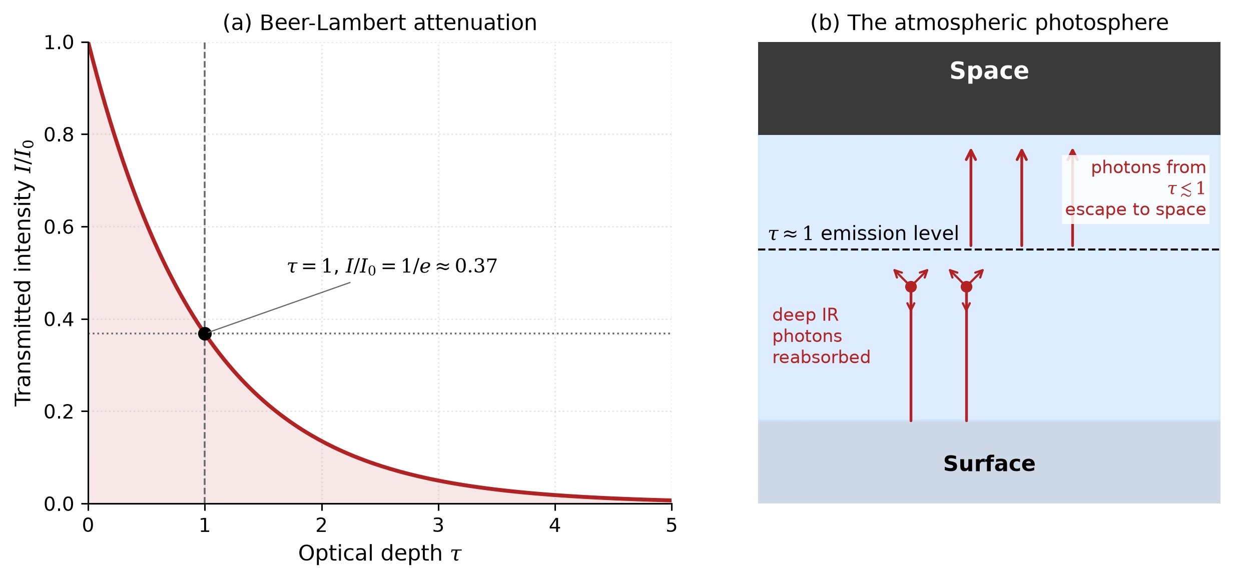
../_images/tau_one_schematic.avif — Fig. 5.20 The atmospheric “photosphere” concept. (a) Beer-Lambert attenuation: the transmitted intensity decreases exponentially with optical depth, \(I/I_0 = e^{-\tau}\) (Eq. (5.8)); the \(\tau = 1\) level transmits a fraction \(1/e \approx 0.37\) of the incident intensity. (b) An infrared photon emitted from deep in the atmosphere (\(\tau \gg 1\)) is absorbed before reaching space and re-emitted in a random direction (the short arrows mark possible re-emission directions); only photons emitted from \(\tau \lesssim 1\) escape freely. The effective emission level at \(\tau \approx 1\) sets the planet’s effective temperature as observed from space. Course-original figure.#

5.6. Energy balance and the greenhouse effect#

5.6.1. Radiative-convective equilibrium#

An atmosphere in which radiation alone carried the energy would not be stable. Near the surface the absorbing gases are optically thick, and the temperature gradient that pure radiative transfer would require there is steeper than the dry adiabat of (5.6). A parcel displaced upward in such a profile remains warmer than its surroundings and keeps rising, so the layer overturns: convection sets in and holds the gradient close to the adiabat. Higher up the atmosphere becomes optically thin, radiation carries the energy efficiently, and the radiative gradient is shallower than the adiabat, so displaced parcels sink back. The tropopause is the level where the two gradients cross. It is therefore an outcome of the energy balance rather than a boundary imposed by hand. This combined state, convective below and radiative above, is called radiative-convective equilibrium, and it is the reason the troposphere and the stratosphere described above behave so differently.

Manabe and Strickler [1964] first solved for such a profile self-consistently in one dimension by computing radiative fluxes for \(\mathrm{H_2O}\), \(\mathrm{CO_2}\), and \(\mathrm{O_3}\) and applying a convective adjustment: wherever the radiative lapse rate exceeded a critical threshold, the profile was adjusted to redistribute energy neutrally. This calculation reproduced both Earth’s surface temperature and tropopause height without prescribing either. Extended to \(\mathrm{CO_2}\)-driven warming [Manabe and Wetherald, 1967], this one-dimensional radiative-convective framework is the direct ancestor of the climate models used for projection today.

Fig. 5.21 sketches this adjustment.

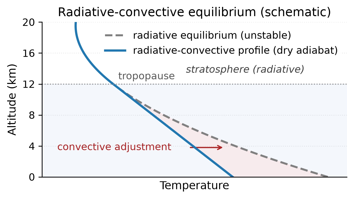
../_images/radiative_convective_profile.avif — Fig. 5.21 Schematic of radiative-convective equilibrium. The dashed grey curve is the temperature profile that pure radiative equilibrium would demand: near the surface its lapse rate exceeds the dry adiabat, so the layer is convectively unstable. Convection overturns the layer and holds the profile (solid blue) on the dry adiabat of about \(9.8\) K km\(^{-1}\) until the two profiles converge at the tropopause; above that level the radiative gradient is shallower than the adiabat and the stratosphere stays radiative. The shaded band marks the convective layer. The temperature axis carries no scale because the diagram is schematic. Course-original figure.#

5.6.2. Planetary energy balance#

Every planet reaches a thermal equilibrium in which the rate of absorbed stellar energy equals the rate of emitted thermal radiation. The stellar flux received at a planet’s orbital distance \(d\) from its star (luminosity \(L_\star\)) is:

(5.9)#\[ F_\star = \frac{L_\star}{4\pi d^2} \]

The planet intercepts this flux over its cross-sectional area \(\pi R_p^2\) and reflects a fraction \(A\) (the Bond albedo). The absorbed power is therefore \((1 - A) \, F_\star \, \pi R_p^2\).

In equilibrium, this absorbed power equals the thermal radiation emitted from the entire surface (\(4\pi R_p^2\)) at the equilibrium temperature \(T_{\mathrm{eq}}\) (also called the effective temperature and written \(T_{\mathrm{eff}}\) in many textbooks) via the Stefan-Boltzmann law (Lecture 3):

\[ (1 - A) \frac{L_\star}{4\pi d^2} \pi R_p^2 = 4\pi R_p^2 \, \sigma \, T_{\mathrm{eq}}^4 \]

Solving for \(T_{\mathrm{eq}}\):

(5.10)#\[ T_{\mathrm{eq}} = \left[\frac{(1-A) \, L_\star}{16 \pi \sigma \, d^2}\right]^{1/4} \]

The equilibrium temperature is the temperature at which a planet radiates if it has no atmosphere (or a completely transparent one), depending only on stellar luminosity, orbital distance, and albedo rather than atmospheric properties.

For Earth, satellite radiometry has measured the individual flux components of the global energy budget to a few W m\(^{-2}\). The leading inventory is from Trenberth et al. [2009] and is shown in Fig. 5.22:

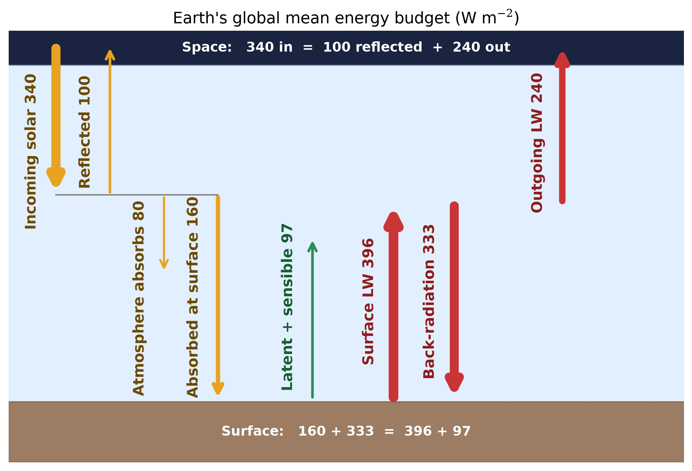
../_images/trenberth_energy_budget.avif — Fig. 5.22 Earth’s globally averaged energy budget in W m\(^{-2}\). Of \(\sim\)340 W m\(^{-2}\) incoming shortwave flux, \(\sim\)100 W m\(^{-2}\) is reflected (Bond albedo \(A \approx 0.30\)), \(\sim\)80 W m\(^{-2}\) is absorbed by the atmosphere, and \(\sim\)160 W m\(^{-2}\) is absorbed at the surface. The surface re-radiates \(\sim\)396 W m\(^{-2}\) in the longwave, while downward back-radiation returns \(\sim\)333 W m\(^{-2}\) as the dominant surface heating term. Latent and sensible heat fluxes (\(\sim\)97 W m\(^{-2}\)) balance surface losses, and top-of-atmosphere balance matches 340 W m\(^{-2}\) incoming to 100 W m\(^{-2}\) reflected plus \(\sim\)240 W m\(^{-2}\) outgoing IR. Schematic adapted from Trenberth *et al.* [2009]. Course-original figure.#

5.6.3. Effective vs. actual surface temperatures#

The table below compares the equilibrium temperature with the measured surface temperature for several solar system bodies:

Body	Albedo \(A\)	\(d\) (AU)	\(T_{\mathrm{eq}}\) (K)	\(T_{\mathrm{surface}}\) (K)	\(\Delta T\) (K)
Venus	0.77	0.72	227	737	+510
Earth	0.30	1.00	255	288	+33
Mars	0.25	1.52	210	215	+5
Jupiter	0.34	5.20	110	165*	+55

*Jupiter’s “surface temperature” refers to the 1-bar level.

The discrepancy \(\Delta T = T_{\mathrm{surface}} - T_{\mathrm{eq}}\) reveals the strength of the greenhouse effect. Venus has a staggering 510 K greenhouse warming, by far the largest in the solar system. Earth’s 33 K greenhouse warming, though modest by comparison, is sufficient to keep the oceans liquid. Mars has only a small greenhouse warming (\(\sim 5\) K) because its \(\mathrm{CO_2}\) atmosphere is very thin (surface pressure only 6 mbar) and lacks the water-vapour amplifier that boosts the warming on Earth and Venus. Jupiter’s excess temperature is partly due to internal heat left over from formation (Lecture 3), not solely the greenhouse effect. The surface temperatures behind these greenhouse contrasts, and the surface pressures of the atmospheres that produce them, are compared for the three terrestrial planets in Fig. 5.23.

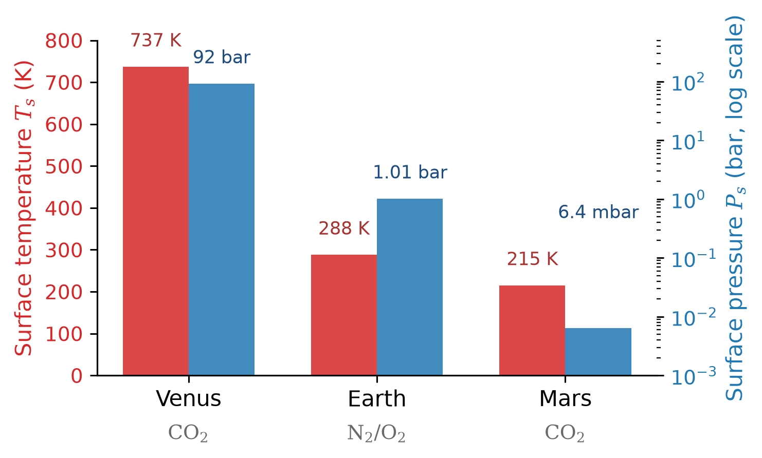
../_images/venus_earth_mars_atmospheres1.avif — Fig. 5.23 Surface temperature (red bars, left axis) and surface pressure (blue bars, right axis, logarithmic) of Venus, Earth and Mars, with the dominant gas of each atmosphere labelled below. Three planets of similar bulk composition span a factor of \(\sim 10^4\) in surface pressure and \(\sim 500\) K in surface temperature. Data from [NASA Jet Propulsion Laboratory, 2026]. Course-original figure.#

5.6.4. The greenhouse mechanism#

The greenhouse effect arises because the atmosphere is relatively transparent to incoming shortwave (visible) radiation from the star but relatively opaque to outgoing longwave (infrared) radiation from the surface. The mechanism works as follows [Pierrehumbert, 2010]:

Sunlight (visible wavelengths, peak \(\sim\)0.5 \(\mu\)m) passes through the atmosphere and heats the surface.
The warm surface emits thermal radiation at infrared wavelengths (peak \(\sim\)10–15 \(\mu\)m for \(T \sim 200\)–\(300\) K).
Greenhouse gases (\(\mathrm{CO_2}\), \(\mathrm{H_2O}\), \(\mathrm{CH_4}\), \(\mathrm{O_3}\), etc.) absorb much of this outgoing IR radiation.
The absorbing layer re-emits IR radiation in all directions: half upward (toward space), half downward (back toward the surface).
The downward emission adds a downward radiative flux at the surface (the atmosphere is not a new energy source: it returns part of what the surface emitted), raising its temperature above \(T_{\mathrm{eq}}\).

The atmospheric absorption spectrum underlying this asymmetry is shown in Fig. 5.24: infrared absorption bands of \(\mathrm{H_2O}\) and \(\mathrm{CO_2}\) block surface emission, leaving an atmospheric window near 8–13 \(\mu\)m.

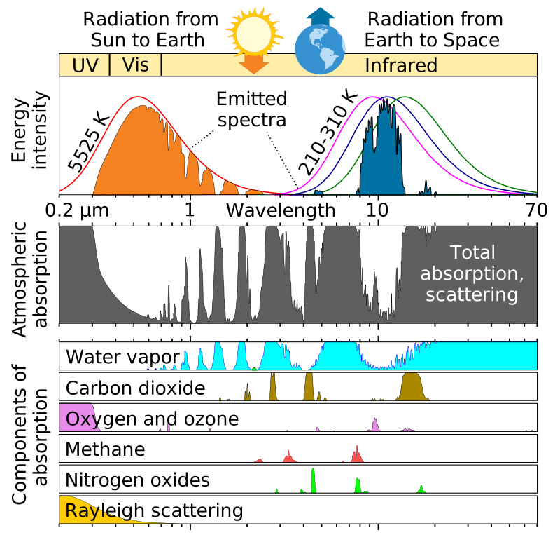
../_images/atmospheric_transmission.svg — Fig. 5.24 Atmospheric absorption spectrum of Earth’s atmosphere from ultraviolet through infrared wavelengths (top: incident solar spectrum; bottom: absorption by individual gases). Infrared absorption bands of \(\mathrm{H_2O}\) and \(\mathrm{CO_2}\) flank the relatively transparent atmospheric window near 8–13 \(\mu\)m. Credit: Wikimedia Commons, public domain.#

5.6.5. One-layer greenhouse model#

We can quantify the greenhouse effect with a simple one-layer model. Consider an atmosphere represented by a single isothermal layer with emissivity \(\varepsilon\) at infrared wavelengths (and completely transparent at visible wavelengths). The energy balance has two components:

Atmospheric layer balance. The layer absorbs a fraction \(\varepsilon\) of the surface emission \(\sigma T_s^4\) and emits \(\varepsilon \sigma T_a^4\) both upward and downward:

(5.11)#\[ \varepsilon \, \sigma \, T_s^4 = 2 \, \varepsilon \, \sigma \, T_a^4 \]

This gives \(T_a^4 = T_s^4 / 2\).

Surface balance. The surface absorbs the incoming stellar flux plus the downward emission from the atmosphere. In equilibrium:

(5.12)#\[ (1-A) \frac{F_\star}{4} + \varepsilon \, \sigma \, T_a^4 = \sigma \, T_s^4 \]

Top-of-atmosphere balance. The planet must radiate to space at its equilibrium temperature, so \((1-A) F_\star / 4 = \sigma T_{\mathrm{eq}}^4\). Combining with the atmospheric and surface balance equations:

(5.13)#\[ T_s = T_{\mathrm{eq}} \left(\frac{2}{2 - \varepsilon}\right)^{1/4} \]

When \(\varepsilon = 0\) (no greenhouse gases), \(T_s = T_{\mathrm{eq}}\): no warming. When \(\varepsilon = 1\) (perfect absorber), \(T_s = 2^{1/4} \, T_{\mathrm{eq}} \approx 1.19 \, T_{\mathrm{eq}}\), a 19% increase in surface temperature. For Earth, this gives \(T_s \approx 1.19 \times 255 \approx 303\) K, a reasonable first estimate, though the real greenhouse effect involves multiple absorbing layers (Fig. 5.25); the breakdown of this balance in the runaway greenhouse is derived in Lecture 9.

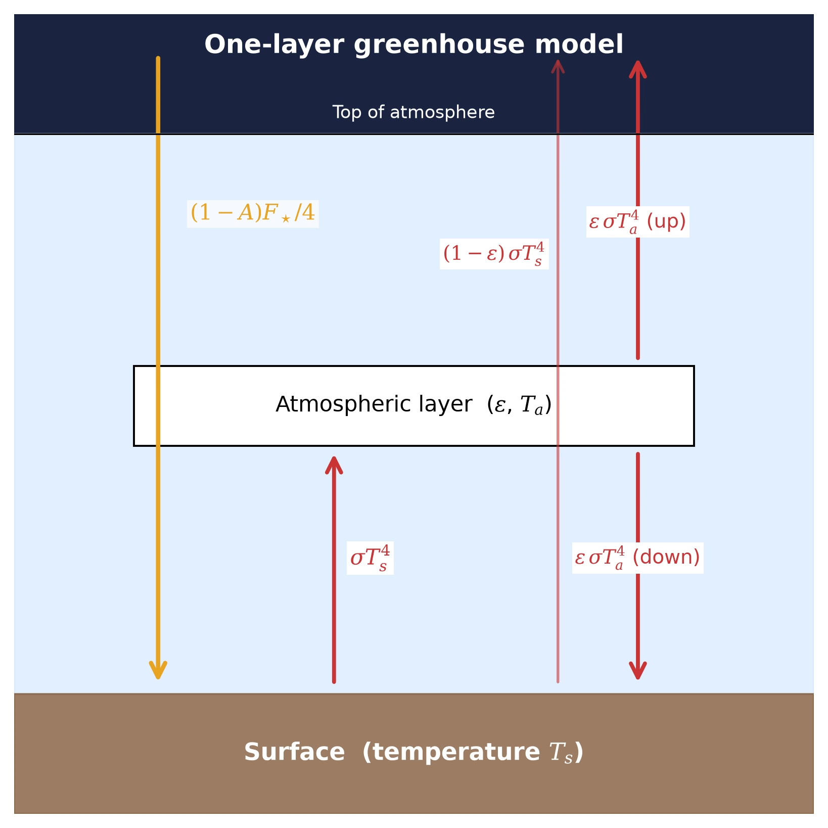
../_images/greenhouse_one_layer.avif — Fig. 5.25 Energy budget of the one-layer greenhouse model. Incident shortwave flux \((1-A)F_\star/4\) is absorbed at the surface, which re-radiates \(\sigma T_s^4\) in the infrared; a fraction \((1-\varepsilon)\) escapes directly to space, while a fraction \(\varepsilon\) is absorbed in the atmospheric layer. The layer re-emits \(\varepsilon\,\sigma T_a^4\) upward to space and downward to the surface, raising \(T_s\) above the equilibrium temperature \(T_\mathrm{eq}\). Schematic following Pierrehumbert [2010]. Course-original figure.#

5.7. Atmospheric escape#

An atmosphere is not permanent. Over geological time, gas molecules can be lost to space through several physical mechanisms. The balance between outgassing supply and escape loss determines a planet’s atmospheric mass and composition over its history [Lammer et al., 2008].

The dominant escape regime for a given planet-species pair depends on two quantities: the Jeans escape parameter \(\lambda_J\) (the ratio of gravitational binding energy to thermal energy at the exobase, the altitude above which the atmosphere becomes collisionless) and the incident EUV flux from the host star (which heats the upper atmosphere and drives bulk outflow). Low \(\lambda_J\) or high EUV flux pushes the system into hydrodynamic outflow, a bulk, wind-like escape of the entire upper atmosphere; high \(\lambda_J\) with low EUV flux corresponds to the retention regime in which escape is negligible on Gyr timescales. Thermal escape is not the only loss channel: the stellar wind and a planetary magnetic field enable or suppress several additional escape processes, summarised in Fig. 5.26.

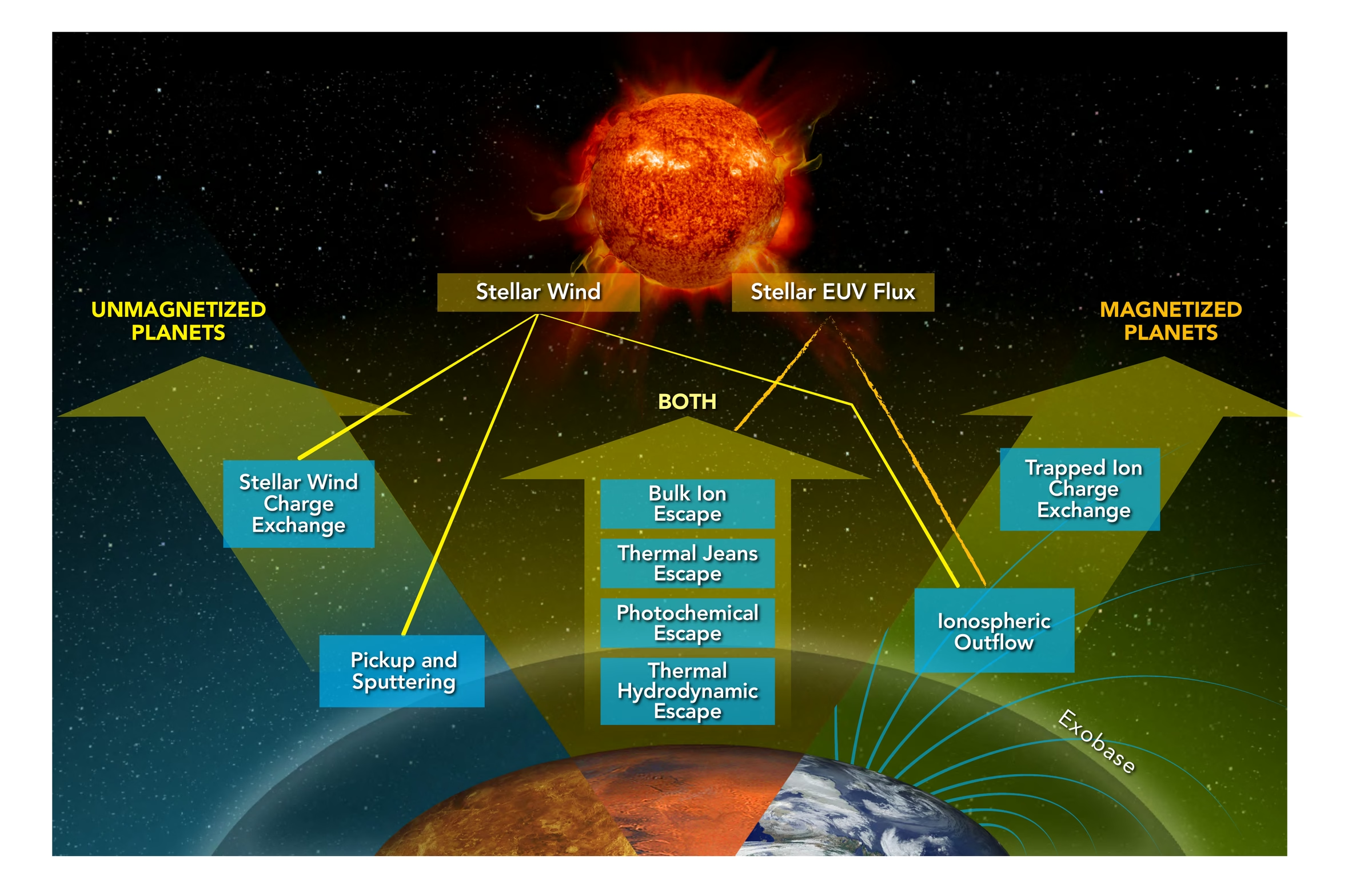
../_images/escape_processes_gronoff2020.avif — Fig. 5.26 Overview of the main atmospheric escape processes and the conditions under which each operates. The central column lists the processes that act on both magnetised and unmagnetised planets, powered mainly by the stellar EUV flux: thermal escape (Jeans and hydrodynamic), photochemical escape, and bulk ion escape. On unmagnetised planets such as Venus and Mars (left), the stellar wind interacts directly with the upper atmosphere and drives sputtering, ion pickup, and charge exchange. On magnetised planets such as Earth (right), the magnetic field deflects the stellar wind but channels ions into ionospheric outflow along open field lines and permits charge exchange of magnetospherically trapped ions. Each process operates either near the exobase, the altitude above which the atmosphere becomes collisionless, or in the extended region above it. Reproduced from Gronoff *et al.* [2020], Fig. 2.#

5.7.1. Thermal (Jeans) escape#

The most fundamental escape mechanism is Jeans escape, which arises from the thermal velocity distribution of gas molecules. In a gas at temperature \(T\), molecules have a range of speeds described by the Maxwell-Boltzmann distribution. The most probable thermal speed is \(v_{\mathrm{th}} = \sqrt{2 \kB T / m}\), where \(m\) is the molecular mass. Most molecules are far too slow to escape, but the tail of the distribution extends to arbitrarily high speeds, and some molecules in this high-velocity tail exceed the escape speed.

The exobase (Fig. 5.27) is the altitude at which the mean free path \(\ell = 1/(n \sigma)\), with \(\sigma\) an effective collision cross-section, equals the pressure scale height \(H\). Below this level, collisions dominate and the gas behaves as a fluid; above it, collisions are rare enough that molecules travel on ballistic trajectories, and those with \(v > v_\mathrm{esc}\) escape to space without further interaction. For Earth, the exobase sits near 500 km altitude; for Mars, closer to 200 km.

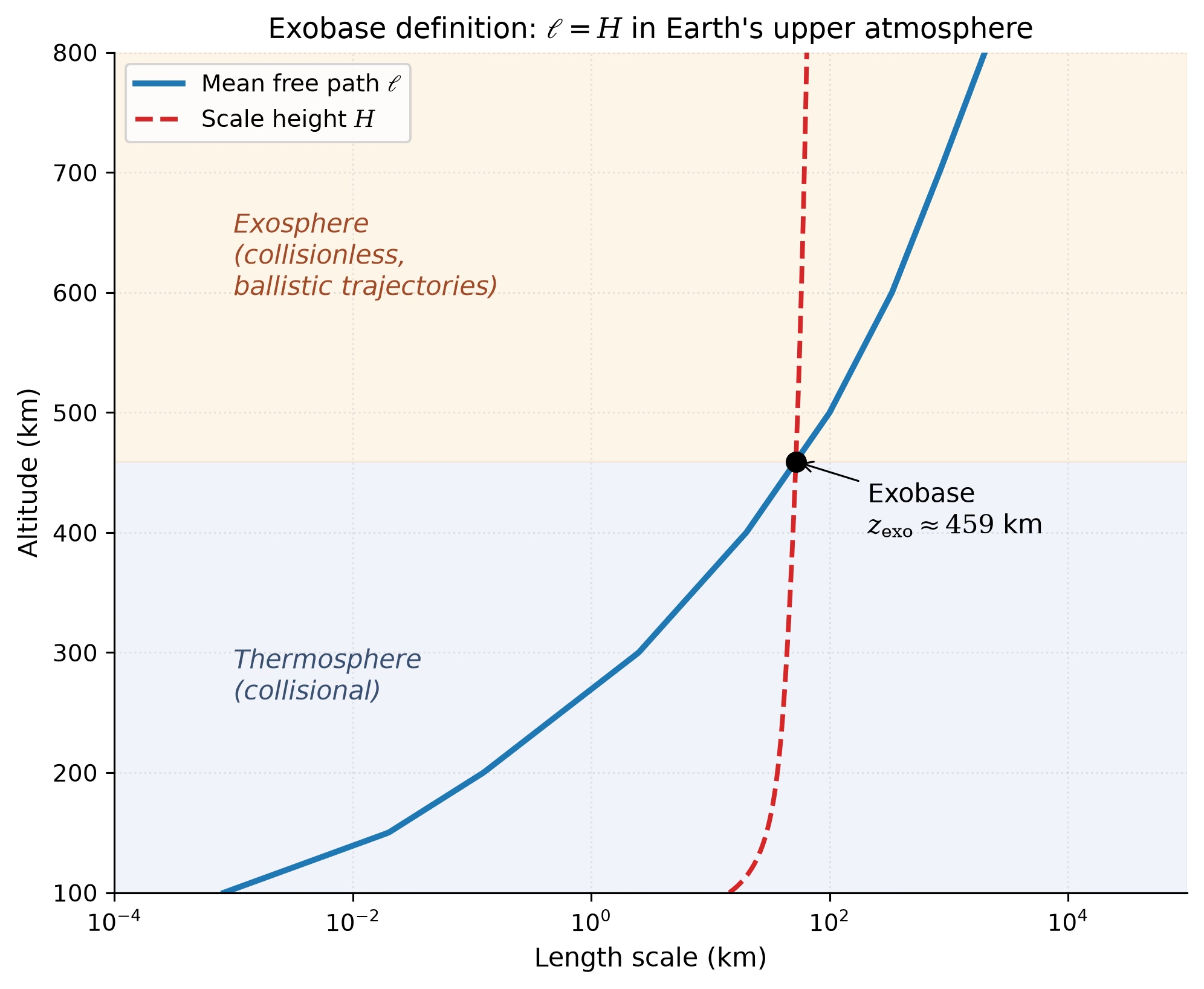
../_images/exobase_definition.avif — Fig. 5.27 The exobase as the altitude where the mean free path \(\ell\) (blue) equals the pressure scale height \(H\) (red dashed) in Earth’s upper atmosphere. Below the crossing (blue shading) the atmosphere is collisional (thermosphere); above it (orange shading) the atmosphere is effectively collisionless (exosphere) and ballistic trajectories carry individual molecules to escape. The crossing altitude is approximately 450 to 500 km for present-day Earth, depending on solar activity and exobase temperature. Number densities follow the US Standard Atmosphere 1976 [NOAA and NASA and U.S. Air Force, 1976] below 86 km, joined to an isothermal thermosphere above (an analytic profile, not an MSIS-86 tabulation); effective cross-section \(\sigma = 10^{-18}\ \mathrm{m}^2\). Course-original figure.#

The key parameter governing Jeans escape is the Jeans escape parameter \(\lambda_J\), defined at the exobase:

(5.14)#\[ \lambda_J = \frac{G M_p \, m}{\kB T_{\mathrm{exo}} \, r_{\mathrm{exo}}} = \frac{v_{\mathrm{esc}}^2}{v_{\mathrm{th}}^2} \]

where \(M_p\) is the planet’s mass, \(m\) is the molecular mass, \(T_{\mathrm{exo}}\) is the exobase temperature, \(r_{\mathrm{exo}}\) is the exobase radius, \(v_{\mathrm{esc}} = \sqrt{2GM_p/r_{\mathrm{exo}}}\) is the escape speed, and \(v_{\mathrm{th}} = \sqrt{2\kB T_{\mathrm{exo}}/m}\) is the most probable thermal speed.

The Jeans escape parameter is the ratio of gravitational binding energy to thermal energy for a molecule at the exobase. When \(\lambda_J \gg 1\), very few molecules have enough energy to escape and escape is slow. When \(\lambda_J \lesssim 2\)–3, a substantial fraction of molecules can escape, and the atmosphere erodes rapidly.

The Jeans escape flux (number of molecules escaping per unit area per unit time from the exobase) is:

(5.15)#\[ \Phi_J = \frac{n_{\mathrm{exo}} \, v_{\mathrm{th}}}{2\sqrt{\pi}} \, (1 + \lambda_J) \, e^{-\lambda_J} \]

where \(n_{\mathrm{exo}}\) is the number density at the exobase. The exponential factor \(e^{-\lambda_J}\) shows that escape is extremely sensitive to \(\lambda_J\): a small change in temperature, gravity, or molecular mass can change the escape rate by orders of magnitude.

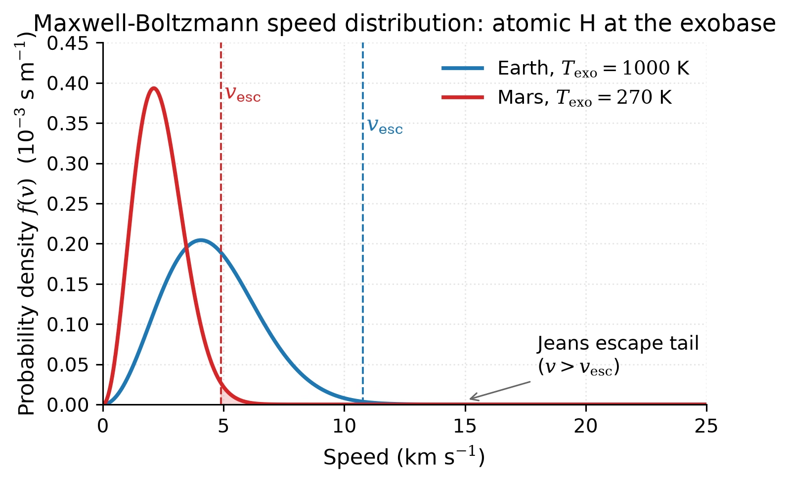
../_images/maxwell_boltzmann_jeans.avif — Fig. 5.28 Maxwell-Boltzmann speed distribution for atomic hydrogen at the exobase temperatures of Earth (\(T_\mathrm{exo} = 1000\) K, blue) and Mars (\(T_\mathrm{exo} = 270\) K, red). Dashed vertical lines mark the escape velocity \(v_\mathrm{esc}\) at the exobase of each planet: 10.8 km s\(^{-1}\) at 500 km altitude for Earth, and 4.9 km s\(^{-1}\) at 200 km altitude for Mars. These are the same exobase altitudes used for the \(\lambda_J\) values tabulated below. Only molecules in the high-speed tail above \(v_\mathrm{esc}\) (shaded) contribute to Jeans escape; the exponential dependence of the tail area on \(\lambda_J = v_\mathrm{esc}^2 / v_\mathrm{th}^2\) explains why escape rates vary by orders of magnitude across species and bodies. Course-original figure.#

The following table illustrates \(\lambda_J\) for several atmospheric species on Earth and Mars, evaluated at the exobase: \(T_\mathrm{exo} = 1000\) K and \(r_\mathrm{exo} = R_\oplus + 500\) km for Earth, \(T_\mathrm{exo} = 270\) K and \(r_\mathrm{exo} = R_M + 200\) km for Mars.

Species	\(m\) (u)	\(\lambda_J\) (Earth)	\(\lambda_J\) (Mars)
H	1	7.0	5.3
\(\mathrm{H_2}\)	2	14	11
He	4	28	21
\(\mathrm{N_2}\)	28	200	150
\(\mathrm{CO_2}\)	44	310	230

For heavy species like \(\mathrm{N_2}\) and \(\mathrm{CO_2}\), \(\lambda_J\) is so large that Jeans escape is negligible on both planets. For atomic hydrogen, \(\lambda_J\) is moderate, leading to measurable escape: this is why both Earth and Mars lose hydrogen to space (Fig. 5.28). Earth’s exobase temperature is not fixed at 1000 K: it varies from \(\sim\)600 K at solar minimum to \(\sim\)1500 K at solar maximum, which modulates the escape flux of the lightest species by orders of magnitude. We will revisit this derivation in full detail (starting from the Maxwell-Boltzmann distribution) in Lecture 10.

5.7.2. Hydrodynamic escape#

When the energy input to the upper atmosphere is very large (for example, from intense extreme ultraviolet (EUV) radiation from a young, active star), the escape can transition from the slow, molecule-by-molecule Jeans process to a bulk hydrodynamic outflow in which the entire upper atmosphere flows outward like a wind (Fig. 5.29). This is analogous to the solar wind but driven by stellar heating rather than the star’s own thermal energy [Hunten et al., 1987].

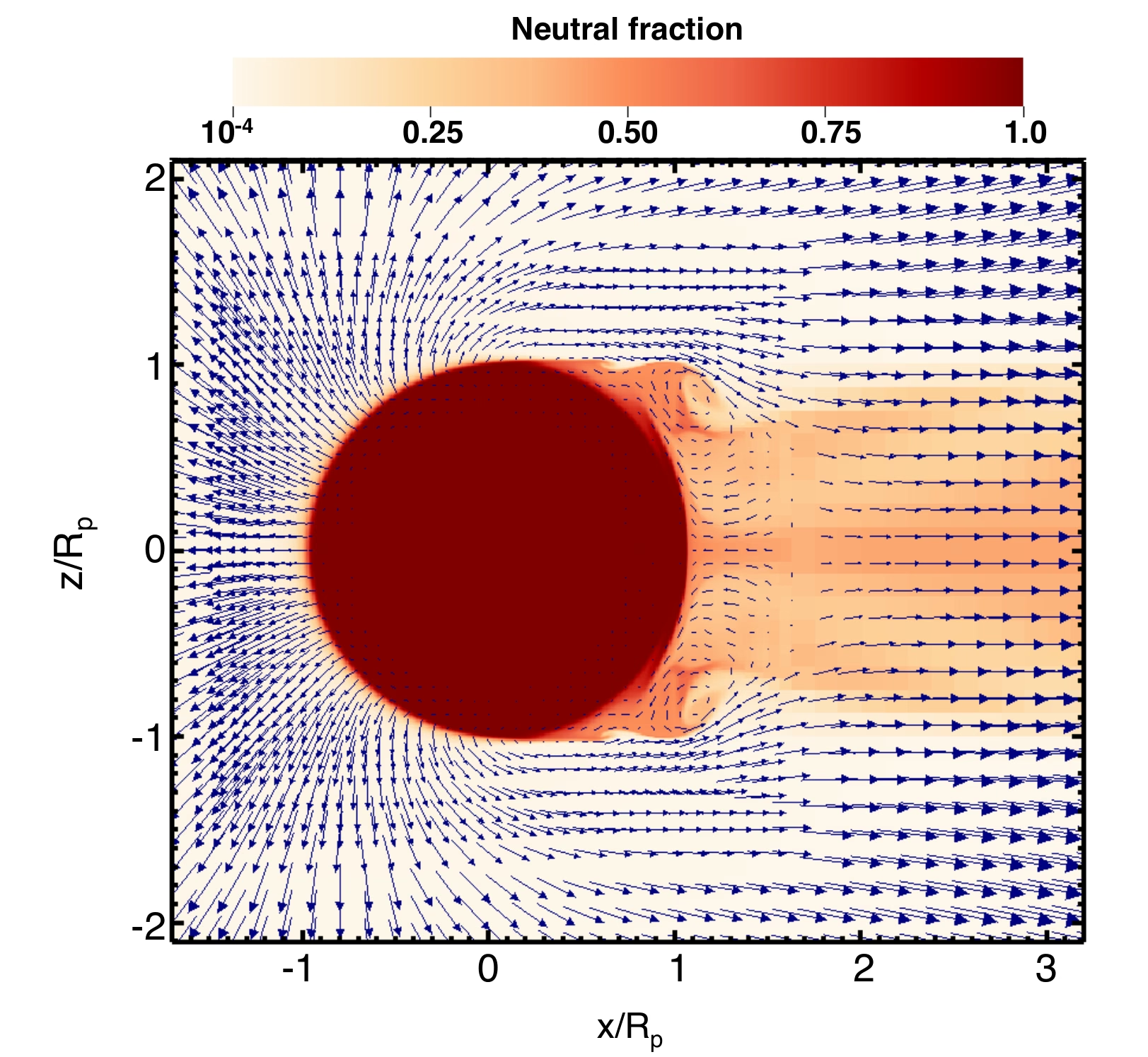
../_images/hot_jupiter_outflow_tripathi2015.avif — Fig. 5.29 Velocity field (arrows) and neutral hydrogen fraction (colour scale) of an EUV-driven hydrodynamic outflow from a hot Jupiter (radius \(2.14\ \Rjup\), mass \(0.53\ \Mjup\)), from the 3D radiation-hydrodynamic simulations of Tripathi *et al.* [2015]. Axes are in units of the planetary radius \(R_p\); the star is to the left. The heated gas accelerates outward from the bound atmosphere (dark red, neutral) and flows around the terminator into a partially neutral wake that flares out on the night side (right). The shear between the day-side wind and the night-side gas produces the Kelvin-Helmholtz rolls visible near \(x \approx 1\,R_p\); away from the planet the outflow is almost fully ionised (light shading). Reproduced from Owen [2019], Fig. 2.#

Hydrodynamic outflows of this kind are observed directly. Ultraviolet transit spectroscopy has detected extended envelopes of escaping atomic hydrogen around the hot Jupiter HD 209458 b [Vidal-Madjar et al., 2003] and the warm Neptune GJ 436 b [Ehrenreich et al., 2015], and near-infrared spectroscopy has revealed escaping helium around the warm super-Neptune WASP-107 b [Spake et al., 2018].

A first estimate of the loss rate in this regime follows from equating the stellar EUV energy absorbed by the upper atmosphere to the gravitational binding energy of the gas that leaves [Watson et al., 1981]. If a fraction \(\eta\) of the incident flux \(F_{\mathrm{EUV}}\) intercepted over the planetary disc goes into lifting material out of the potential well, the energy-limited mass-loss rate is

(5.16)#\[ \dot{M}_{\mathrm{EL}} = \eta \, \frac{\pi \, F_{\mathrm{EUV}} \, R_p^3}{G \, M_p} \]

with \(\eta \approx 0.1-0.2\) for hydrogen-dominated atmospheres. Two scalings matter most. The rate rises as \(R_p^3\), so an extended, low-density envelope is stripped far faster than a compact one, and it falls as \(1/M_p\), so a low surface gravity makes escape easier. Equation (5.16) holds only while the absorbed energy is spent on the outflow. When the gas is dense enough, the ions and electrons that the EUV photons create recombine before the gas can flow out. The gas then loses energy as radiation, through recombination-continuum photons and Lyman \(\alpha\), and these photons leave the atmosphere. Most of the deposited energy then radiates away instead of lifting gas, and the true loss rate falls below this estimate [Owen, 2019].

Hydrodynamic escape is most important during a planet’s first few hundred million years, when the host star’s EUV luminosity is 10–100 times higher than at present, stripping hydrogen-rich primary atmospheres to produce the observed exoplanet radius valley between \(\sim\)1.5 and \(2 \, \Rearth\) (Fig. 5.31) [Fulton et al., 2017] (Lecture 13).

Fig. 5.30 shows a population synthesis in which this escape carves the valley into the radius distribution.

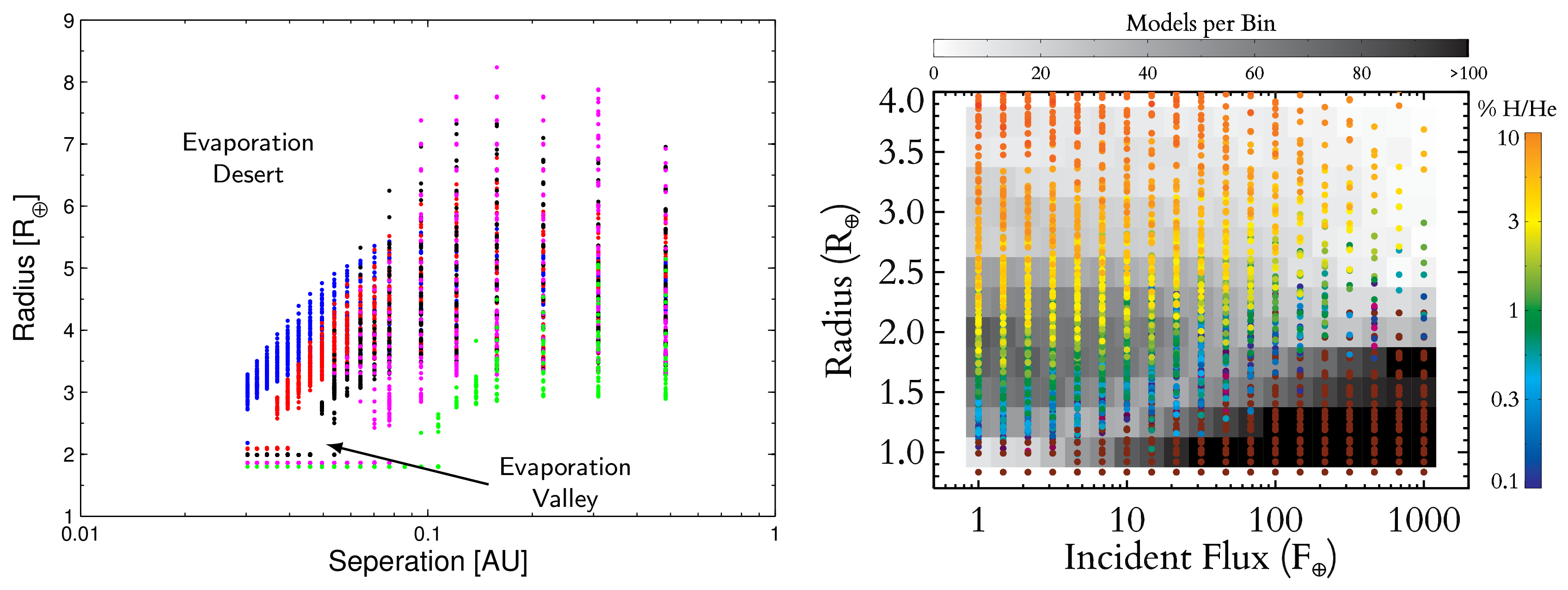
../_images/radius_valley_owen2019.avif — Fig. 5.30 Population synthesis of close-in exoplanets that have undergone EUV-driven hydrodynamic atmospheric escape. *Left*: planet radius vs orbital separation after 10 Gyr of evolution, for cores with masses 6.5 to 15 \(\Mearth\) (blue 15, red 12.5, black 10, magenta 7.5, green 6.5 \(\Mearth\); the published axis label reads “Seperation” [sic] in the original figure). The “evaporation desert” at small separations and large radii is empty because all H/He envelopes have been stripped, and the “evaporation valley” appears as a thin gap near \(1.5\!-\!2\,\Rearth\). *Right*: planet radius vs incident bolometric flux (\(F_\oplus\), in units of Earth’s), colour-coded by retained atmospheric mass fraction (% H/He). Greyscale shading shows the number of models per bin. Left panel from Owen and Wu [2013], right panel from Lopez and Fortney [2013]; the desert and valley labels follow Owen [2019], Fig. 3.#

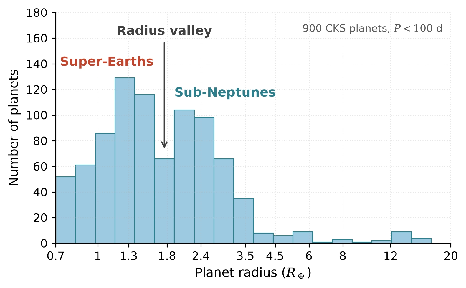
../_images/fulton2017_radius_valley.avif — Fig. 5.31 Observed radius distribution of short-period (\(P < 100\) days) small planets from the California-Kepler Survey [Fulton *et al.*, 2017]. Two distinct populations appear: a super-Earth peak near \(1.3\ \Rearth\) (likely stripped rocky cores) and a sub-Neptune peak near \(2.4\ \Rearth\) (cores with retained H/He envelopes of a few percent by mass). The gap between them near \(1.8\ \Rearth\) is the observational signature of the radius valley predicted by photoevaporation models. Course figure: raw counts of the 900 CKS planets with \(P < 100\) days in logarithmic radius bins, drawn from Table 2 of Fulton *et al.* [2017]; no completeness correction is applied, which the paper adds before it measures the occurrence per star, so the valley here is the observed deficit and the counts below about \(1.1\ \Rearth\) are lowered by the survey’s incompleteness for small planets.#

The outflowing hydrogen can also drag heavier species along with it, which fractionates the atmosphere that remains [Hunten et al., 1987].

5.7.3. Non-thermal escape mechanisms#

Several processes can eject atmospheric particles to space without relying on thermal energy [Lammer et al., 2008]:

Sputtering: Energetic ions from the solar wind or magnetospheric plasma impact the upper atmosphere and transfer enough momentum to eject atmospheric molecules. This is significant for Mars, which lacks a global magnetic field to deflect the solar wind.
Photochemical escape: Solar UV radiation dissociates molecules (e.g., \(\mathrm{H_2O} \to\) H + OH), producing fast atoms with enough energy to escape. This is an important loss channel for hydrogen from Venus and Mars.
Ion pickup: Atmospheric atoms ionised by solar UV or charge exchange are picked up by the solar wind magnetic field and swept away from the planet. This process is particularly effective at unmagnetised planets like Mars and Venus.
Impact erosion: Large asteroid or comet impacts can eject a large fraction of a planet’s atmosphere. The efficiency depends on the impactor size relative to the atmospheric scale height: very large impacts can blow off a substantial atmospheric mass in a single event.

The MAVEN mission at Mars has measured the present-day total atmospheric escape rate at \(\sim 2\)–\(3\) kg s\(^{-1}\) for H and O combined across photochemical, thermal, and solar-wind-driven channels (Fig. 5.34) [Jakosky et al., 2018] (Lecture 10).

Fig. 5.32 shows the orbit from which MAVEN samples the upper atmosphere, with a periapsis near 150 km.

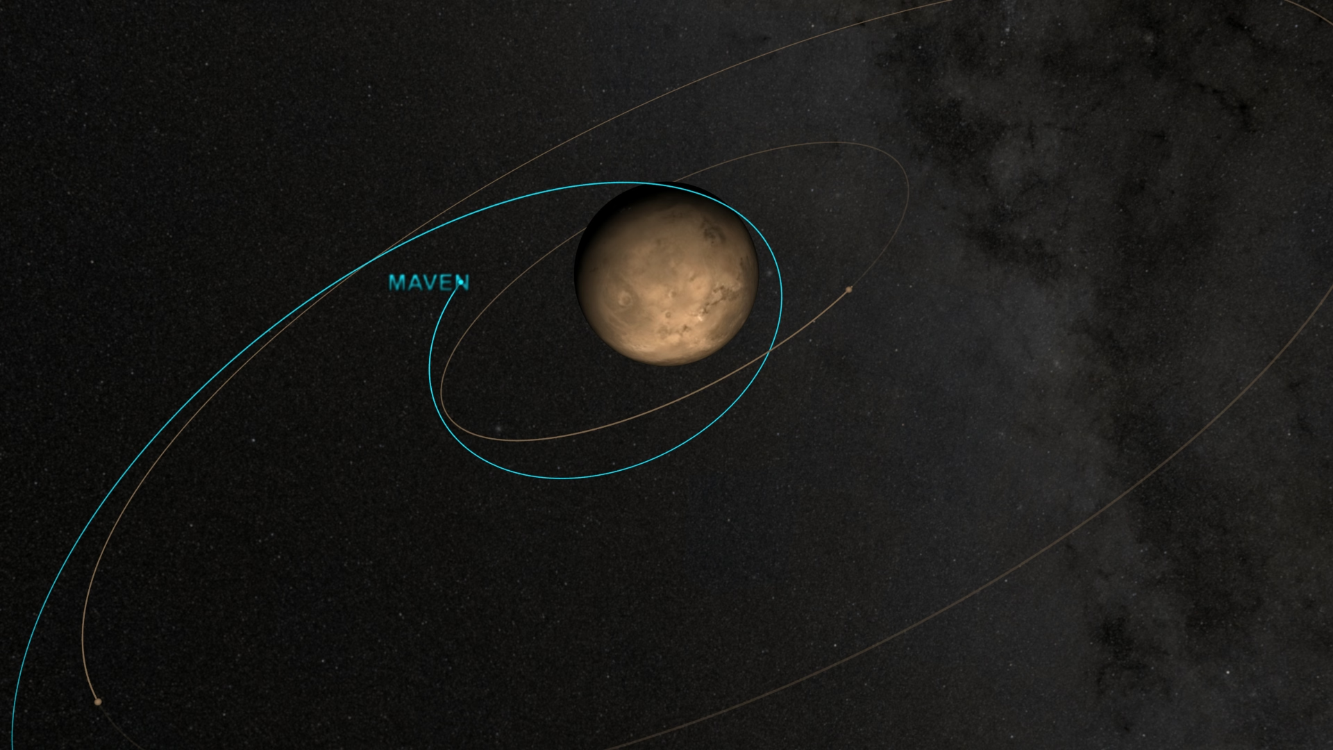
../_images/maven_science_orbit.avif — Fig. 5.32 MAVEN’s science orbit around Mars, showing how the spacecraft transitioned from the highly elliptical Mars-orbit insertion trajectory (outermost path) through an intermediate ellipse to its final science orbit with a periapsis near \(\sim\)150 km altitude and an apoapsis of \(\sim\)6200 km. The low-altitude periapsis passes sample the thermosphere and exobase region where most species-specific escape occurs, while the higher apoapsis samples the ionised tail and pickup-ion environment downstream of Mars relative to the solar wind. The combination enables simultaneous in-situ and remote-sensing characterisation of the atmospheric-escape pathways summarised above. Credit: NASA’s Scientific Visualization Studio (SVS ID 4190), public domain.#

Fig. 5.33 shows the resulting picture of ion escape: the most energetic ions leave in a plume above the planet, the bulk along the tail.

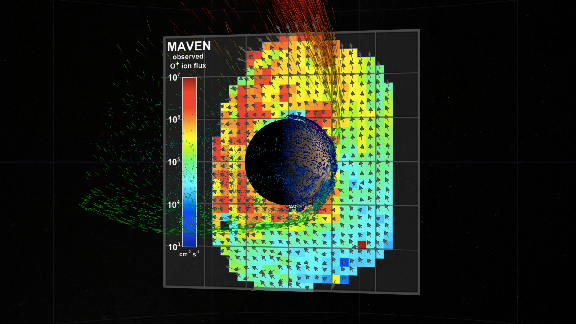
../_images/maven_ion_plume.avif — Fig. 5.33 NASA Scientific Visualization Studio rendering of the ion plume escaping from Mars, based on MAVEN data. The most energetic ions (red) are accelerated in a plume above the planet, while the bulk of escaping ions (green) are lost along the tail region behind Mars relative to the solar wind. Unmagnetised Mars is particularly vulnerable to this class of solar-wind-driven escape because the solar wind reaches deep into the upper atmosphere rather than being deflected by a global dipole field. Credit: NASA’s Scientific Visualization Studio (SVS ID 4370), PI Bruce Jakosky, public domain.#

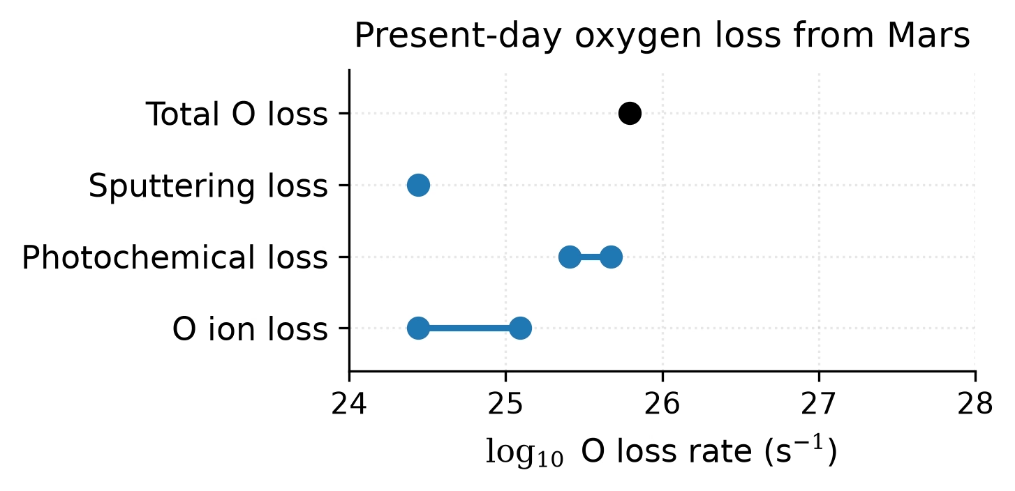
../_images/maven_o_loss_channels.avif — Fig. 5.34 Present-day oxygen loss rates from Mars decomposed into escape channels, after Jakosky *et al.* [2018] Fig. 6. Markers give the loss rate (log\(_{10}\) of the number of O atoms per second) for O ion escape, photochemical escape, and sputtering, plus the combined total; a bar spans the published range of a channel. Photochemical escape dominates the oxygen budget today; sputtering is sub-dominant at present solar activity but was likely comparable or larger in the young, EUV-active Sun epoch. The total is drawn as its own marker; the three channels add up to it in linear units, and together with hydrogen escape they give the \(\sim 2\)–\(3\) kg s\(^{-1}\) figure quoted in the text. Course-original figure.#

5.8. Atmospheric retention#

Whether a planet retains its atmosphere over billions of years depends on the competition between escape processes and atmospheric sources (outgassing, volatile delivery). The outcome is controlled primarily by two parameters: the planet’s escape velocity and the thermal velocity of atmospheric molecules.

5.8.1. The escape velocity–temperature diagram#

The classic tool for assessing atmospheric retention is a plot of escape velocity versus surface (or exosphere) temperature. Each atmospheric species occupies a characteristic region based on its thermal velocity \(v_{\mathrm{th}} = \sqrt{2\kB T / m}\). The rule of thumb for long-term retention is [de Pater and Lissauer, 2010]:

\[ v_{\mathrm{esc}} \gtrsim 6 \, v_{\mathrm{th}} \]

A planet retains a given gas species if its escape velocity exceeds roughly 6 times the thermal velocity of that species (corresponding to \(\lambda_J \gtrsim 36\), which keeps Jeans escape negligible over billions of years).

5.8.2. Solar system trends#

Applying this criterion reveals a clear pattern across the solar system:

Gas giants (Jupiter, Saturn): With escape velocities of 60 and 36 km s\(^{-1}\) respectively, and moderate exosphere temperatures, they retain all species, including the lightest (\(\mathrm{H_2}\), He). This is why they still possess their primary atmospheres.
Earth and Venus: Escape velocities of \(\sim\)11 km s\(^{-1}\) are sufficient to retain heavy molecules (\(\mathrm{N_2}\), \(\mathrm{O_2}\), \(\mathrm{CO_2}\), \(\mathrm{H_2O}\)) but not atomic hydrogen. Earth and Venus lose H to space, which contributes to long-term water loss (via photodissociation of \(\mathrm{H_2O}\) followed by H escape).
Mars: With \(v_{\mathrm{esc}} = 5.0\) km s\(^{-1}\) and an exosphere temperature of \(\sim\)270 K, Mars holds \(\mathrm{CO_2}\) firmly against thermal escape (\(\lambda_J \approx 230\)) and is marginal only for lighter species such as \(\mathrm{H_2O}\) and \(\mathrm{N_2}\). While Jeans escape of \(\mathrm{CO_2}\) is negligible, non-thermal processes (sputtering, ion pickup) have eroded most of Mars’s original atmosphere over 4 billion years [Jakosky et al., 2018].
Titan: Despite its low escape velocity (2.6 km s\(^{-1}\)), Titan retains a thick \(\mathrm{N_2}\) atmosphere because it is extremely cold (\(T_{\mathrm{exo}} \approx 150\) K). Low temperature means low thermal velocities, and the Jeans parameter remains large for \(\mathrm{N_2}\); the hydrogen that methane photochemistry produces in the upper atmosphere has \(\lambda_J\) of order a few and leaks away to space.
Moon and Mercury: With escape velocities of 2.4 and 4.3 km s\(^{-1}\) and high dayside temperatures (\(>\)400 K), these bodies cannot retain any significant atmosphere. Mercury has only a tenuous exosphere (a collisionless atmosphere with surface pressure \(\sim 10^{-15}\) bar).

The classic graphical summary of these competing constraints is the escape-velocity-vs-temperature diagram (Fig. 5.35).

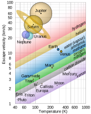
../_images/escape_velocity_temperature.svg — Fig. 5.35 Escape velocity versus surface temperature for solar system bodies. Diagonal lines indicate the thermal velocity of different gas species (scaled by a factor of 6 for long-term retention). Bodies above and to the left of a species line can retain that gas; bodies below and to the right cannot. The gas giants retain everything; Earth and Venus retain heavy species but lose H; Mars and Titan are marginal; the Moon and Mercury retain essentially nothing. Credit: Wikimedia Commons, CC BY-SA 4.0.#

5.8.3. Atmospheric evolution over time#

Atmospheric retention is not simply a present-day snapshot: it evolves over a planet’s lifetime [Lammer et al., 2008]:

Young stars are UV-bright: Stars emit 10–100 times more EUV in their first few hundred million years, driving hydrodynamic escape that can strip primary atmospheres from low-mass planets.
Magnetic field loss: A planet that loses its global magnetic field (like Mars \(\sim\)4 Gyr ago; Lecture 4) becomes exposed to solar wind sputtering and ion pickup, accelerating atmospheric loss.
Outgassing replenishment: Continuous volcanic outgassing of \(\mathrm{CO_2}\), \(\mathrm{H_2O}\), and \(\mathrm{SO_2}\) replenishes atmospheric gases on geologically active planets with vigorous interior convection.
Atmospheric chemistry: Solar UV dissociates \(\mathrm{H_2O}\) into escaping H and rock-sequestered O, the leading hypothesis for the loss of Venus’s primordial water inventory.

We examine these evolutionary pathways in detail for Venus’s runaway greenhouse (Lecture 9), Mars’s atmospheric collapse (Lecture 10), and exoplanetary atmospheres (Lecture 13).

Mars shows the combined outcome: the thin haze on its limb in Fig. 5.36 is what remains after 4 Gyr of escape from a small planet without a global magnetic field.

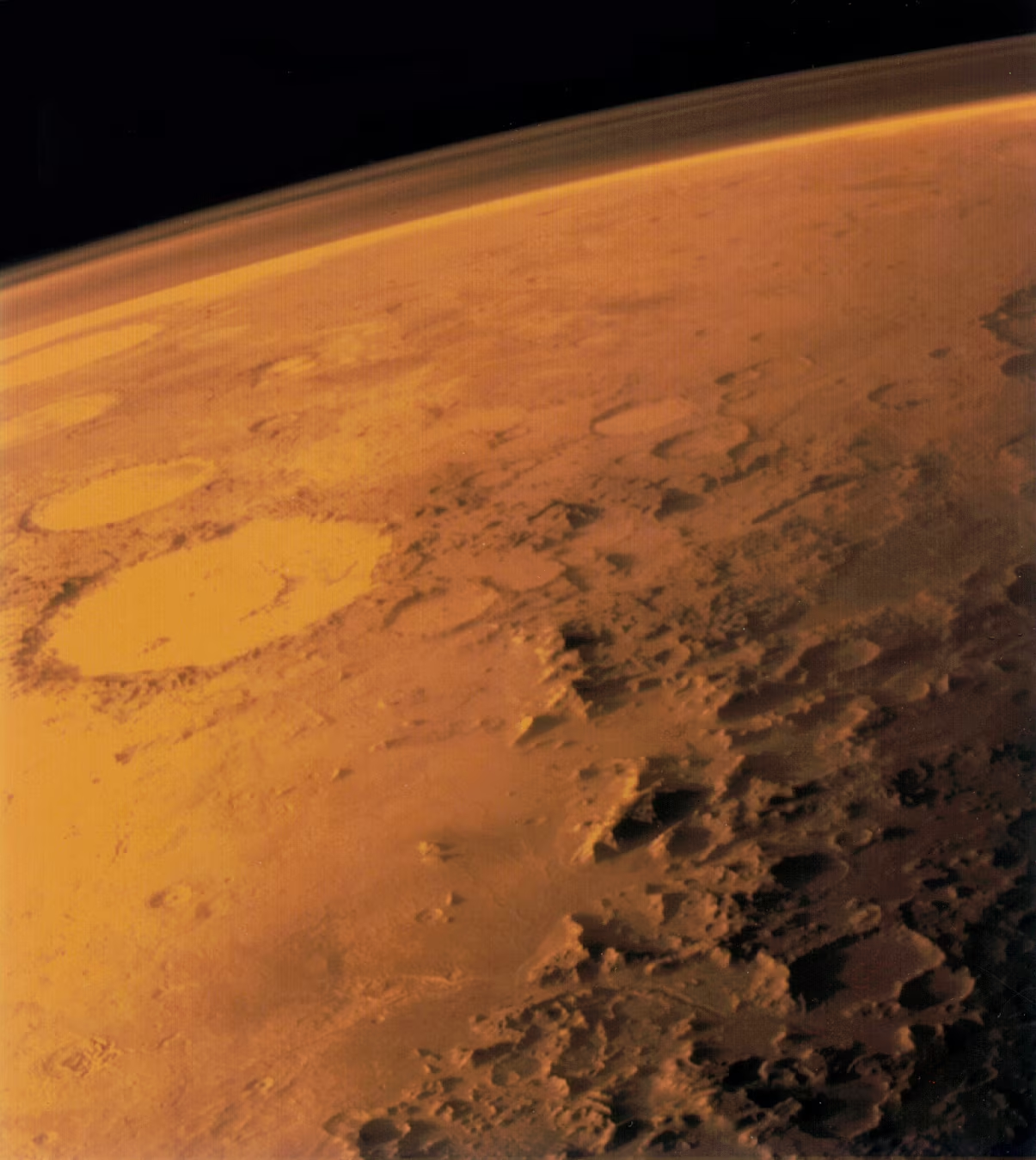
../_images/mars_atmosphere.avif — Fig. 5.36 The Martian atmosphere visible as a thin haze layer on the limb, photographed by NASA’s *Viking 1* orbiter in 1976. With a surface pressure of only 6 mbar (\(\sim\)0.6% of Earth’s), Mars’s atmosphere is too thin to sustain liquid water or provide significant greenhouse warming today. Geological evidence for ancient rivers, lakes, and possibly an ocean indicates that Mars once had a much thicker atmosphere, most of which has been lost to space over the past \(\sim\)4 billion years through solar wind stripping and other escape processes. Credit: NASA/JPL, public domain.#

5.9. Recent advances#

The James Webb Space Telescope (JWST) has opened a new era in exoplanet atmospheric characterisation. Thermal emission measurements of TRAPPIST-1 b, an Earth-sized planet orbiting an M dwarf, indicate a dayside temperature consistent with bare rock and no significant atmosphere (Fig. 5.38) [Greene et al., 2023]. Similar results for TRAPPIST-1 c [Zieba et al., 2023] suggest that innermost rocky planets around active M dwarfs may be stripped of their atmospheres by intense stellar irradiation [Wordsworth and Kreidberg, 2022]. Prolonged stellar irradiation during the extended high-activity saturated regime of M dwarfs (during which X-ray and EUV output stays at a fixed fraction of the bolometric luminosity: a few hundred Myr for a Sun-like star, but beyond 1 Gyr for a mid-M dwarf, Fig. 5.37) drives sustained escape that can strip secondary atmospheres from close-in rocky worlds (Lecture 13, Lecture 14).

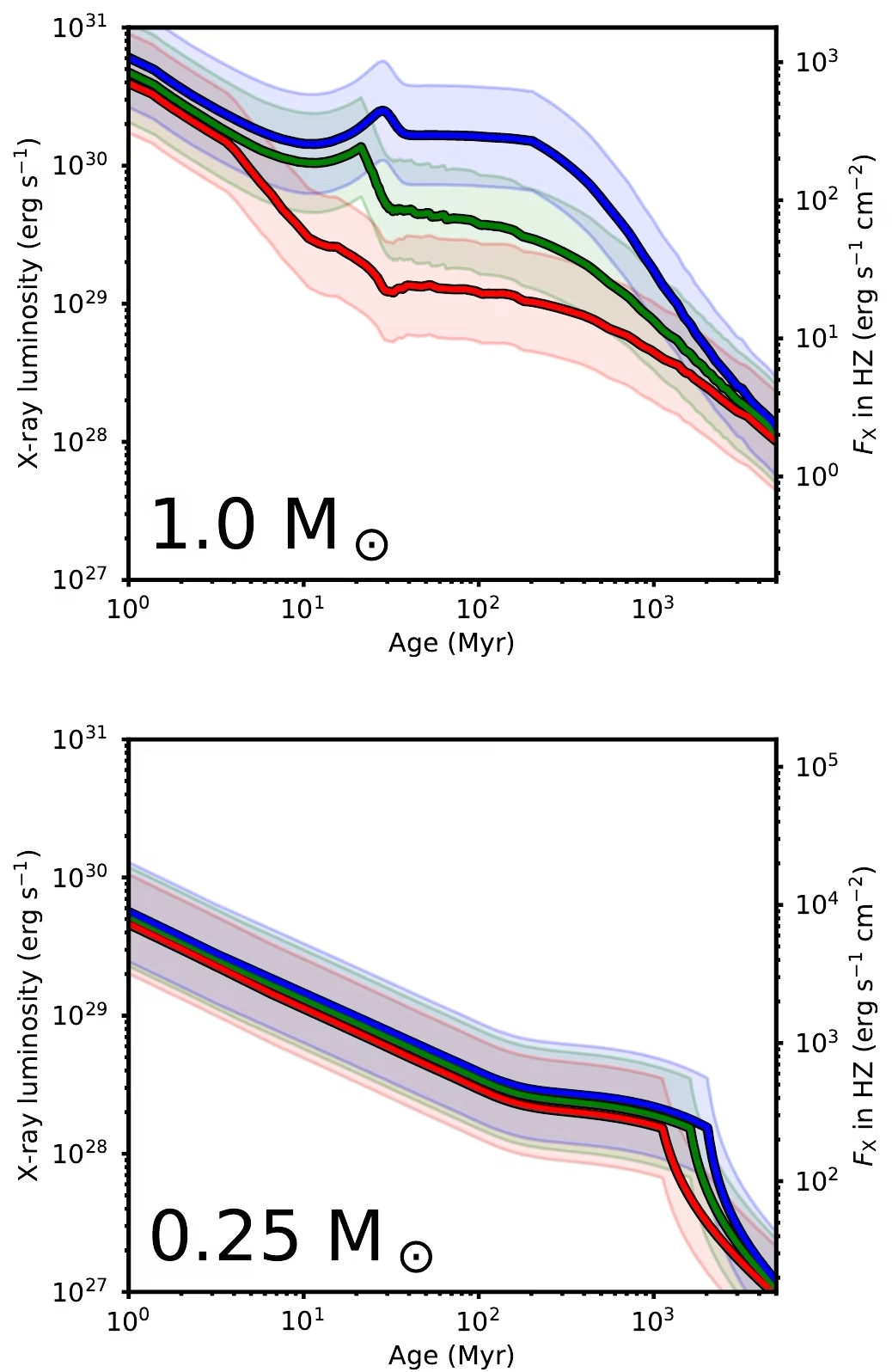
../_images/johnstone2021_xuv_evolution.avif — Fig. 5.37 Evolutionary tracks for stellar X-ray luminosity for slow, medium, and fast rotators (red, green and blue lines; faster rotators stay active longer) for a Sun-like star (1.0 \(M_\odot\), top) and a mid-M dwarf (0.25 \(M_\odot\), bottom). Shaded bands give one standard deviation around the mean track. Lower-mass stars remain in the saturated regime \(L_X / L_\mathrm{bol} \sim 10^{-3}\) for far longer than Sun-like stars: \(\sim 100\) Myr for \(1.0\,M_\odot\), \(\gtrsim 1\) Gyr for \(0.25\,M_\odot\). Close-in rocky planets around late-M stars (e.g. the TRAPPIST-1 system) therefore experience prolonged high-XUV irradiation that drives sustained atmospheric escape. Reproduced from [Johnstone *et al.*, 2021], Fig. 11 (two of the four stellar-mass panels shown).#

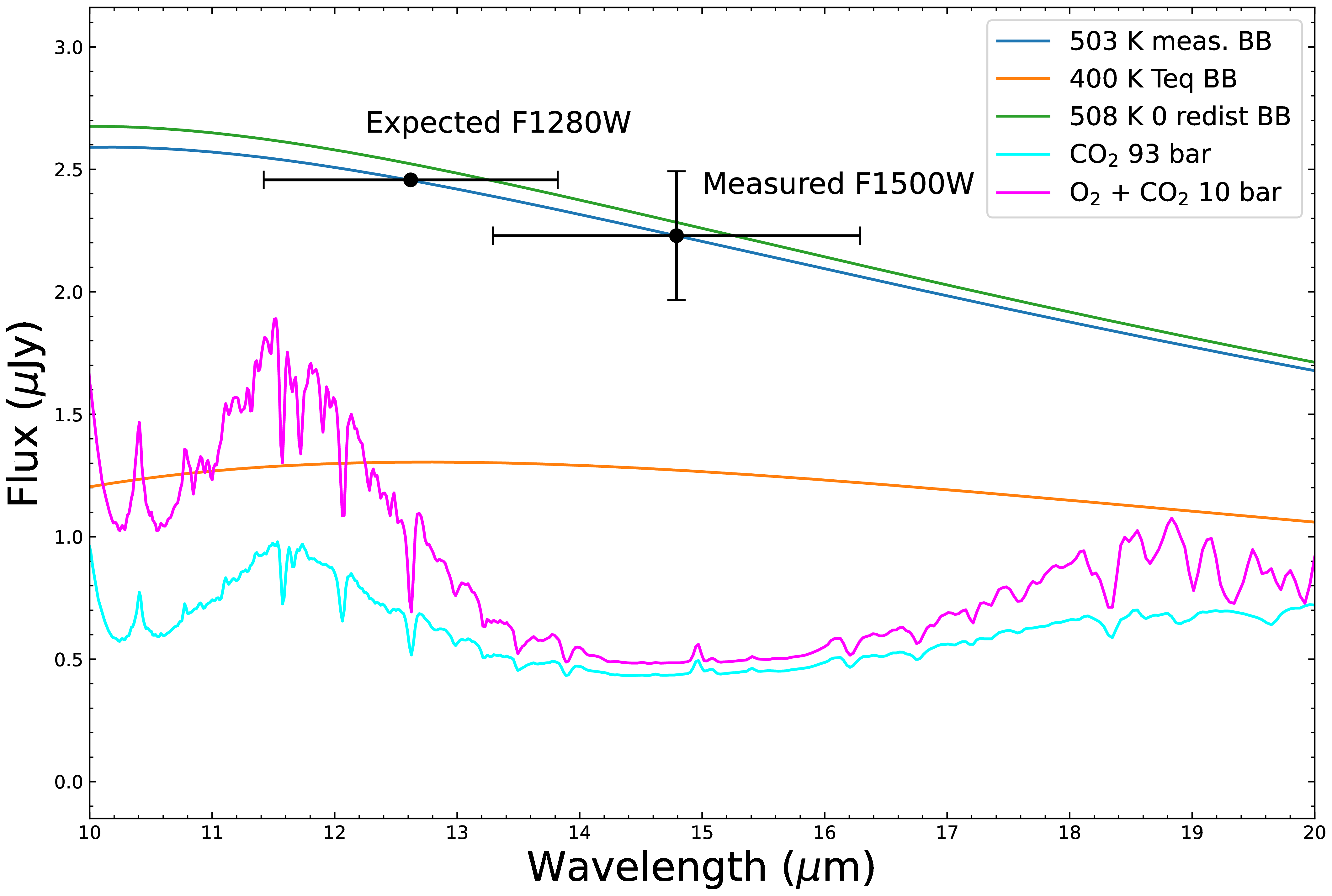
../_images/trappist1b_jwst_greene2023.avif — Fig. 5.38 JWST/MIRI 15 \(\mu\)m thermal emission measurement of TRAPPIST-1 b (black point with error bars labelled “Measured F1500W”) compared with predicted spectra. The measured dayside flux matches a bare-rock blackbody at \(T_B = 503\) K (blue curve), close to the 508 K blackbody predicted for zero heat redistribution and no atmosphere (green curve), and is significantly above the 400 K isotropic-redistribution blackbody (orange) that would be expected for an efficient atmospheric heat engine. The second black point (“Expected F1280W”) marks the flux the bare-rock fit predicts in the neighbouring 12.8 \(\mu\)m band. Thick atmospheres (e.g. 93 bar \(\mathrm{CO_2}\), cyan; 10 bar \(\mathrm{O_2}/\mathrm{CO_2}\), magenta) absorb in the 15 \(\mu\)m band and would suppress the observed flux by a factor of two or more, inconsistent with the data. The result is best explained by little-to-no redistribution from a thin or absent atmosphere on the dayside of TRAPPIST-1 b. Figure from Greene *et al.* [2023].#

5.10. Looking ahead to Lecture 6#

This lecture treated an atmosphere as a static column: its composition, vertical structure, and energy budget. Lecture 6 sets that column in motion. Condensation turns vapour into clouds, rotation organises circulation cells and jets, and feedbacks between temperature, ice, and radiation govern climate stability. The hydrostatic and radiative principles established here underpin each of those processes.

5.11. References#

[Catling2017] (1,2,3)

Catling, David C. and Kasting, James F. 2017. Atmospheric Evolution on Inhabited and Lifeless Worlds. Cambridge University Press, Cambridge. doi:10.1017/9781139020558.

[dePaterLissauer2010] (1,2)

de Pater, Imke and Lissauer, Jack J. 2010. Planetary Sciences. Cambridge University Press, Cambridge, 2nd edition. doi:10.1017/cbo9780511780561.

[Ehrenreich2015]

Ehrenreich, David, Bourrier, Vincent, Wheatley, Peter J., Lecavelier des Etangs, Alain, Hébrard, Guillaume, Udry, Stéphane, Bonfils, Xavier, Delfosse, Xavier, Désert, Jean-Michel, Sing, David K., and Vidal-Madjar, Alfred. 2015. “A giant comet-like cloud of hydrogen escaping the warm Neptune-mass exoplanet GJ 436b.” Nature, 522:459–461. doi:10.1038/nature14501, arXiv:1506.07541, https://ui.adsabs.harvard.edu/abs/2015Natur.522..459E/abstract.

[Fulchignoni2005]

Fulchignoni, M., Ferri, F., Angrilli, F., Ball, A. J., Bar-Nun, A., Barucci, M. A., Bettanini, C., Bianchini, G., Borucki, W., Colombatti, G., Coradini, M., Coustenis, A., Debei, S., Falkner, P., Fanti, G., Flamini, E., Gaborit, V., Grard, R., Hamelin, M., Harri, A. M., Hathi, B., Jernej, I., Leese, M. R., Lehto, A., Lion Stoppato, P. F., López-Moreno, J. J., Mäkinen, T., McDonnell, J. A. M., McKay, C. P., Molina-Cuberos, G., Neubauer, F. M., Pirronello, V., Rodrigo, R., Saggin, B., Schwingenschuh, K., Seiff, A., Simoes, F., Svedhem, H., Tokano, T., Towner, M. C., Trautner, R., Withers, P., and Zarnecki, J. C. 2005. “In situ measurements of the physical characteristics of Titan's environment.” Nature, 438(7069):785–791. doi:10.1038/nature04314, https://ui.adsabs.harvard.edu/abs/2005Natur.438..785F/abstract.

[Fulton2017] (1,2,3)

Fulton, Benjamin J., Petigura, Erik A., Howard, Andrew W., Isaacson, Howard, Marcy, Geoffrey W., Cargile, Phillip A., Hebb, Leslie, Weiss, Lauren M., Johnson, John Asher, Morton, Timothy D., and others. 2017. “The California-Kepler Survey. III. a gap in the radius distribution of small planets.” The Astronomical Journal, 154(3):109. doi:10.3847/1538-3881/aa80eb, arXiv:1703.10375, https://ui.adsabs.harvard.edu/abs/2017AJ....154..109F/abstract.

[Greene2023] (1,2)

Greene, Thomas P., Bell, Taylor J., Ducrot, Elsa, Dyrek, Achrène, Lagage, Pierre-Olivier, and Fortney, Jonathan J. 2023. “Thermal emission from the Earth-sized exoplanet TRAPPIST-1 b using JWST.” Nature, 618(7963):39–42. doi:10.1038/s41586-023-05951-7, arXiv:2303.14849, https://ui.adsabs.harvard.edu/abs/2023Natur.618...39G/abstract.

[Gronoff2020]

Gronoff, G., Arras, P., Baraka, S., Bell, J. M., Cessateur, G., Cohen, O., Curry, S. M., Drake, J. J., Elrod, M., Erwin, J., Garcia-Sage, K., Garraffo, C., Glocer, A., Heavens, N. G., Lovato, K., Maggiolo, R., Parkinson, C. D., Simon Wedlund, C., Weimer, D. R., and Moore, W. B. 2020. “Atmospheric escape processes and planetary atmospheric evolution.” Journal of Geophysical Research: Space Physics, 125:e2019JA027639. doi:10.1029/2019JA027639, https://ui.adsabs.harvard.edu/abs/2020JGRA..12527639G/abstract.

[Helled2014]

Helled, Ravit, Bodenheimer, Peter, Podolak, Morris, Boley, Aaron, Meru, Farzana, Nayakshin, Sergei, Fortney, Jonathan J., Mayer, Lucio, Alibert, Yann, and Boss, Alan P. 2014. “Giant planet formation, evolution, and internal structure.” In Beuther, Henrik, Klessen, Ralf S., Dullemond, Cornelis P., and Henning, Thomas, editors, Protostars and Planets VI, pages 643–665. University of Arizona Press. doi:10.2458/azu_uapress_9780816531240-ch028, arXiv:1311.1142, https://ui.adsabs.harvard.edu/abs/2014prpl.conf..643H/abstract.

[Hirschmann2012]

Hirschmann, Marc M. 2012. “Magma ocean influence on early atmosphere mass and composition.” Earth and Planetary Science Letters, 341–344:48–57. doi:10.1016/j.epsl.2012.06.015, https://ui.adsabs.harvard.edu/abs/2012E&PSL.341...48H/abstract.

[Hunten1987] (1,2)

Hunten, Donald M., Pepin, Robert O., and Walker, James C. G. 1987. “Mass fractionation in hydrodynamic escape.” Icarus, 69(3):532–549. doi:10.1016/0019-1035(87)90022-4, https://ui.adsabs.harvard.edu/abs/1987Icar...69..532H/abstract.

[Jakosky2018] (1,2,3)

Jakosky, Bruce M., Brain, David, Chaffin, Michael, Curry, Shannon, Deighan, Justin, Grebowsky, Joseph, Halekas, Jasper, Leblanc, François, Lillis, Robert, Luhmann, Janet G., Andersson, Laila, Bougher, Stephen, Eparvier, Francis, Elrod, Meredith, Ergun, Robert, Lo, Daniel, Mcfadden, James, Mitchell, David, and Yelle, Roger. 2018. “Loss of the Martian atmosphere to space: Present-day loss rates determined from MAVEN observations and integrated loss through history.” Icarus, 315:146–157. doi:10.1016/j.icarus.2018.05.030, https://ui.adsabs.harvard.edu/abs/2018Icar..315..146J/abstract.

[Johnstone2021]

Johnstone, C. P., Bartel, M., and Güdel, M. 2021. “The active lives of stars: a complete description of the rotation and XUV evolution of F, G, K, and M dwarfs.” Astronomy & Astrophysics, 649:A96. doi:10.1051/0004-6361/202038407, https://ui.adsabs.harvard.edu/abs/2021A%26A...649A..96J/abstract.

[Krijt2023]

Krijt, Sebastiaan, Kama, Mihkel, McClure, Melissa, Teske, Johanna, Bergin, Edwin A., Shorttle, Oliver, Walsh, Kevin J., and Raymond, Sean N. 2023. “Chemical habitability: supply and retention of life's essential elements during planet formation.” In Inutsuka, Shu-ichiro, Aikawa, Yuri, Muto, Takayuki, Tomida, Kengo, and Tamura, Motohide, editors, Protostars and Planets VII. ASP Conference Series. doi:10.48550/arXiv.2203.10056, arXiv:2203.10056, https://ui.adsabs.harvard.edu/abs/2023ASPC..534.1031K/abstract.

[Lammer2008] (1,2,3)

Lammer, Helmut, Kasting, James F., Chassefière, Eric, Johnson, Robert E., Kulikov, Yuri N., and Tian, Feng. 2008. “Atmospheric escape and evolution of terrestrial planets and satellites.” Space Science Reviews, 139(1–4):399–436. doi:10.1007/s11214-008-9413-5, https://ui.adsabs.harvard.edu/abs/2008SSRv..139..399L/abstract.

[Lissauer2009]

Lissauer, Jack J., Hubickyj, Olenka, D'Angelo, Gennaro, and Bodenheimer, Peter. 2009. “Models of Jupiter's growth incorporating thermal and hydrodynamic constraints.” Icarus, 199(2):338–350. doi:10.1016/j.icarus.2008.10.004, arXiv:0810.5186, https://ui.adsabs.harvard.edu/abs/2009Icar..199..338L/abstract.

[LopezFortney2013]

Lopez, Eric D. and Fortney, Jonathan J. 2013. “The role of core mass in controlling evaporation: the Kepler radius distribution and the Kepler-36 density dichotomy.” The Astrophysical Journal, 776:2. doi:10.1088/0004-637X/776/1/2, arXiv:1305.0269, https://ui.adsabs.harvard.edu/abs/2013ApJ...776....2L/abstract.

[Lyons2014]

Lyons, Timothy W., Reinhard, Christopher T., and Planavsky, Noah J. 2014. “The rise of oxygen in Earth's early ocean and atmosphere.” Nature, 506(7488):307–315. doi:10.1038/nature13068, https://ui.adsabs.harvard.edu/abs/2014Natur.506..307L/abstract.

[Manabe1964]

Manabe, Syukuro and Strickler, Robert F. 1964. “Thermal equilibrium of the atmosphere with a convective adjustment.” Journal of the Atmospheric Sciences, 21:361–385. doi:10.1175/1520-0469(1964)021<0361:TEOTAW>2.0.CO;2, https://ui.adsabs.harvard.edu/abs/1964JAtS...21..361M/abstract.

[Manabe1967]

Manabe, Syukuro and Wetherald, Richard T. 1967. “Thermal equilibrium of the atmosphere with a given distribution of relative humidity.” Journal of the Atmospheric Sciences, 24:241–259. doi:10.1175/1520-0469(1967)024<0241:TEOTAW>2.0.CO;2, https://ui.adsabs.harvard.edu/abs/1967JAtS...24..241M/abstract.

[Nicholls2024]

Nicholls, Harrison, Lichtenberg, Tim, Bower, Dan J., and Pierrehumbert, Raymond. 2024. “Magma ocean evolution at arbitrary redox state.” Journal of Geophysical Research: Planets, 129:e2024JE008576. doi:10.1029/2024JE008576, https://doi.org/10.1029/2024JE008576.

[Owen2019] (1,2,3)

Owen, James E. 2019. “Atmospheric escape and the evolution of close-in exoplanets.” Annual Review of Earth and Planetary Sciences, 47:67–90. doi:10.1146/annurev-earth-053018-060246, arXiv:1807.07609, https://ui.adsabs.harvard.edu/abs/2019AREPS..47...67O/abstract.

[OwenWu2013]

Owen, James E. and Wu, Yanqin. 2013. “Kepler planets: a tale of evaporation.” The Astrophysical Journal, 775(2):105. doi:10.1088/0004-637X/775/2/105, arXiv:1206.2367, https://ui.adsabs.harvard.edu/abs/2013ApJ...775..105O/abstract.

[Pierrehumbert2010] (1,2,3)

Pierrehumbert, Raymond T. 2010. Principles of Planetary Climate. Cambridge University Press, Cambridge. doi:10.1017/CBO9780511780783.

[Robinson2014] (1,2,3)

Robinson, T. D. and Catling, D. C. 2014. “Common 0.1 bar tropopause in thick atmospheres set by pressure-dependent infrared transparency.” Nature Geoscience, 7(1):12–15. doi:10.1038/ngeo2020, arXiv:1312.6859, https://ui.adsabs.harvard.edu/abs/2014NatGe...7...12R/abstract.

[Seiff1985]

Seiff, A., Schofield, J. T., Kliore, A. J., Taylor, F. W., Limaye, S. S., Revercomb, H. E., Sromovsky, L. A., Kerzhanovich, V. V., Moroz, V. I., and Marov, M. Ya. 1985. “Models of the structure of the atmosphere of Venus from the surface to 100 kilometers altitude.” Advances in Space Research, 5(11):3–58. doi:10.1016/0273-1177(85)90197-8, https://ui.adsabs.harvard.edu/abs/1985AdSpR...5...3S/abstract.

[Spake2018]

Spake, J. J., Sing, D. K., Evans, T. M., Oklopčić, A., Bourrier, V., Kreidberg, L., Rackham, B. V., Irwin, P. G. J., Ehrenreich, D., Wyttenbach, A., and others. 2018. “Helium in the eroding atmosphere of an exoplanet.” Nature, 557:68–70. doi:10.1038/s41586-018-0067-5, arXiv:1805.01298, https://ui.adsabs.harvard.edu/abs/2018Natur.557...68S/abstract.

[Tellmann2009]

Tellmann, Silvia, Pätzold, Martin, Häusler, Bernd, Bird, Michael K., and Tyler, G. Leonard. 2009. “Structure of the Venus neutral atmosphere as observed by the radio science experiment VeRa on Venus Express.” Journal of Geophysical Research: Planets, 114(E9):E00B36. doi:10.1029/2008JE003204, https://ui.adsabs.harvard.edu/abs/2009JGRE..114.0B36T/abstract.

[Trenberth2009] (1,2)

Trenberth, Kevin E., Fasullo, John T., and Kiehl, Jeffrey. 2009. “Earth's global energy budget.” Bulletin of the American Meteorological Society, 90(3):311–324. doi:10.1175/2008BAMS2634.1, https://journals.ametsoc.org/view/journals/bams/90/3/2008bams2634_1.xml.

[Tripathi2015]

Tripathi, Anjali, Kratter, Kaitlin M., Murray-Clay, Ruth A., and Krumholz, Mark R. 2015. “Simulated photoevaporative mass loss from hot Jupiters in 3D.” The Astrophysical Journal, 808(2):173. doi:10.1088/0004-637X/808/2/173, https://ui.adsabs.harvard.edu/abs/2015ApJ...808..173T/abstract.

[VidalMadjar2003]

Vidal-Madjar, A., Lecavelier des Etangs, A., Désert, J.-M., Ballester, G. E., Ferlet, R., Hébrard, G., and Mayor, M. 2003. “An extended upper atmosphere around the extrasolar planet HD209458b.” Nature, 422:143–146. doi:10.1038/nature01448, https://ui.adsabs.harvard.edu/abs/2003Natur.422..143V/abstract.

[Watson1981]

Watson, Andrew J., Donahue, Thomas M., and Walker, James C. G. 1981. “The dynamics of a rapidly escaping atmosphere: applications to the evolution of Earth and Venus.” Icarus, 48:150–166. doi:10.1016/0019-1035(81)90101-9, https://ui.adsabs.harvard.edu/abs/1981Icar...48..150W/abstract.

[Wordsworth2022]

Wordsworth, Robin and Kreidberg, Laura. 2022. “Atmospheres of rocky exoplanets.” Annual Review of Astronomy and Astrophysics, 60:159–201. doi:10.1146/annurev-astro-052920-125632, arXiv:2112.04663, https://ui.adsabs.harvard.edu/abs/2022ARA%26A..60..159W/abstract.

[Zieba2023]

Zieba, Sebastian, Kreidberg, Laura, Ducrot, Elsa, Gillon, Michaël, Morley, Caroline, Schaefer, Laura, Tamburo, Patrick, Koll, Daniel D. B., Lustig-Yaeger, Jacob, Lyu, Renyu, and others. 2023. “No thick carbon dioxide atmosphere on the rocky exoplanet TRAPPIST-1 c.” Nature, 620(7975):746–749. doi:10.1038/s41586-023-06232-z, arXiv:2306.10150, https://ui.adsabs.harvard.edu/abs/2023Natur.620..746Z/abstract.

[NASAFactSheet] (1,2,3)

NASA Jet Propulsion Laboratory. 2026. Planetary physical parameters. NASA Solar System Dynamics, Caltech/JPL. Values derive from the IAU/IAG Working Group report (Archinal et al. 2018, Celestial Mechanics and Dynamical Astronomy 130:22) and current GM estimates. https://ssd.jpl.nasa.gov/planets/phys_par.html.

[USStandardAtmosphere1976] (1,2,3)

NOAA and NASA and U.S. Air Force. 1976. U.s. standard atmosphere, 1976. Technical Report NOAA-S/T 76-1562, National Oceanic and Atmospheric Administration, National Aeronautics and Space Administration, United States Air Force, Washington, D.C. U.S. Government Printing Office, public domain.