14. Synthesis, Solar System in Context & Astrobiology

Learning objectives: By the end of this lecture, you will be able to place our solar system within the observed exoplanet population, evaluate habitability as a coupled systems-level property rather than a single condition, derive the classical habitable-zone boundaries from stellar luminosity and the liquid-water condition, and identify the most promising targets and biggest open questions for life-detection efforts in the coming decade.

See also

Slides: Download Lecture 14 (PDF)

14.1. Part 1: The solar system in the exoplanet context

14.1.1. Recap: what this course has shown

Thirteen lectures have built a single argument from the bottom up. Lectures 1 to 8 introduced protoplanetary disks, interior evolution and differentiation, atmospheres, surfaces, and internal structure. Lectures 9 to 12 walked the solar system body by body: Earth and Venus (Lecture 9), Mercury and Mars (Lecture 10), the gas and ice giants (Lecture 11), and small-body populations (Lecture 12), surveying the overall architecture of our planetary system (Fig. 14.1). Lecture 13 showed how the same physics applies to several thousand planetary systems detected since 1995 [Mayor and Queloz, 1995].

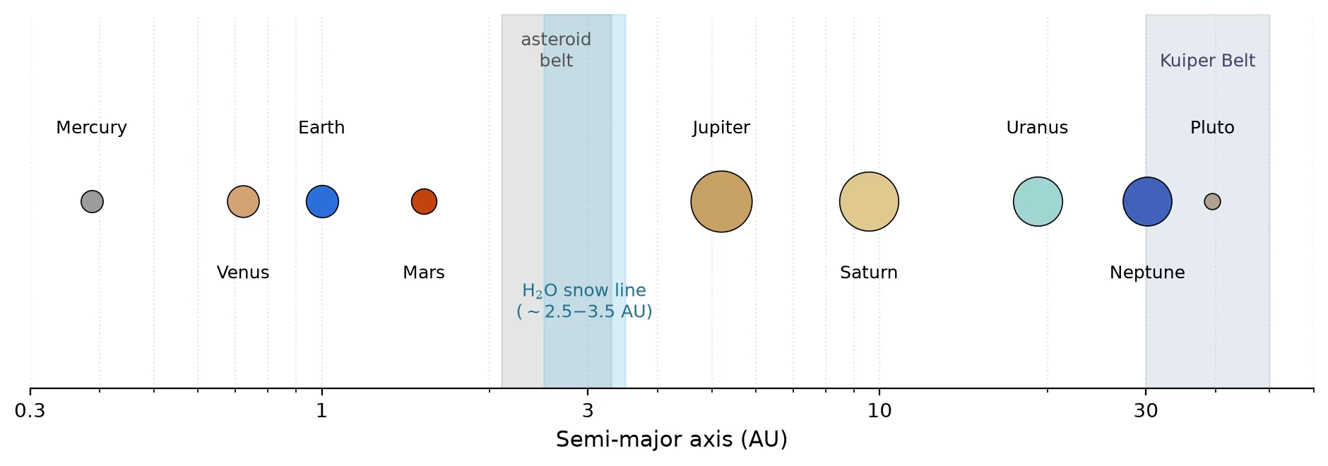
Fig. 14.1 Architecture of the Solar System on a logarithmic semi-major-axis scale. The eight planets and Pluto are drawn with symbol area scaled as \(\log(1 + R/\Rearth)\) so that all bodies remain visible; shaded spans mark the asteroid main belt (\(2.1\) to \(3.3\) AU), the classical Kuiper Belt (\(30\) to \(50\) AU), and the \(2.5\) to \(3.5\) AU range in which the solar nebula’s water snow line lay, separating the rocky inner planets from the gas and ice giants. Semi-major axes and radii from Williams [2026]. Course-original figure.

The thread is simple: physical processes shape planetary outcomes everywhere. The diversity of planets in the galaxy, and the differences between Earth, Venus, and Mars, reflect the same physical processes operating across a wide range of boundary conditions.

This final lecture provides the synthesis. Part 1 places the solar system inside the exoplanet population, identifying where it is typical and where it is atypical. Part 2 reframes habitability as a coupled systems property, in which star, orbit, interior, atmosphere, surface, and biosphere all feed back on one another. Part 3 turns to astrobiology: what we would look for, where we should look, and how confident we can be in the answers. The blackboard derivation reconstructs the classical habitable zone from energy balance, closing with a wrap-up of the course as a whole.

14.1.2. Planet formation theory meets observation

The earlier lectures built the theory of planet formation one stage at a time. This section compares its main predictions with the three kinds of evidence now available: images of disks in which planets form, isotopic dating of the building blocks of the solar system, and the demographics of exoplanets.

Dust in disks coagulates into pebbles forming planetesimals, bodies from roughly a kilometre across produced by the streaming instability. Accreting pebbles and planetesimals build cores that trigger runaway gas accretion [Drążkowska et al., 2023] (Fig. 14.2; Lecture 2).

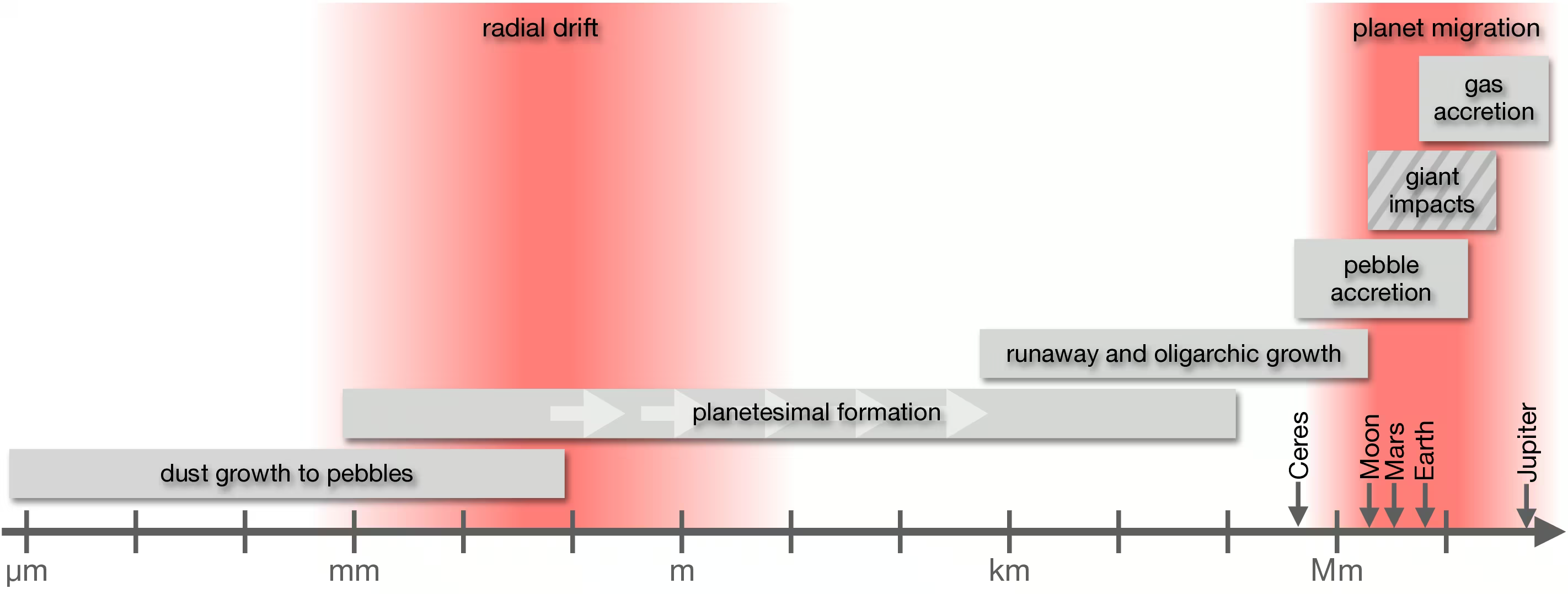
Fig. 14.2 Overview of the dust-to-planet growth processes operating in protoplanetary disks. Dust grains coagulate into pebbles whose radial drift can either be halted at pressure traps (planetesimal formation via the streaming instability) or accreted directly onto growing embryos. Larger embryos compete via runaway and oligarchic growth and, once massive enough, trigger gas envelope accretion. Reproduced from Drążkowska et al. [2023].

Mass growth curves for cores growing by pebble versus planetesimal accretion are shown in Fig. 14.3.

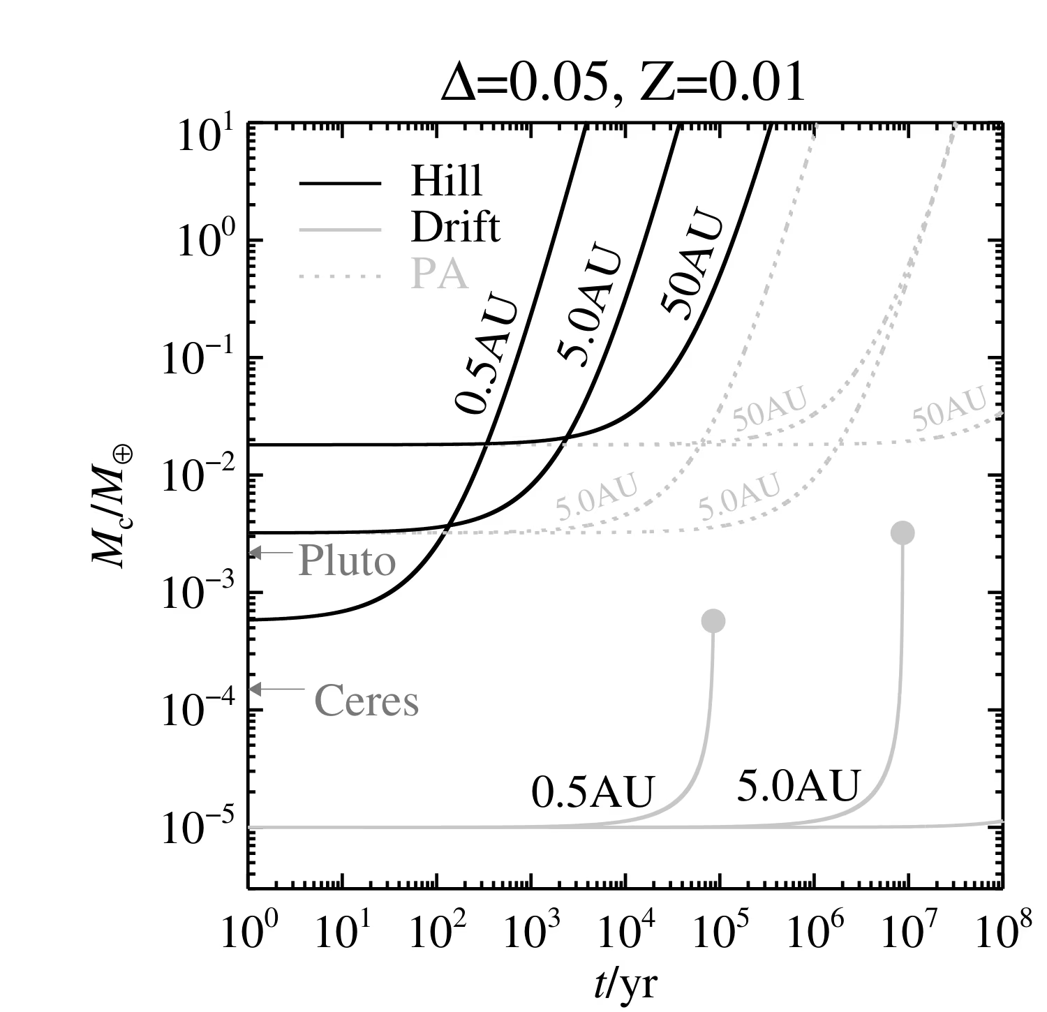
Fig. 14.3 Mass growth of a planetary core as a function of time at three orbital radii (0.5, 5, and 50 AU), from Lambrechts and Johansen [2012] Fig. 11. Grey solid lines show pebble accretion in the drift regime from \(10^{-5}\) Earth masses up to the transition mass (grey dot); black lines show the faster Hill regime, drawn from the transition mass at \(t = 0\) rather than from the end of the drift phase. Grey dotted lines show classical planetesimal accretion, the faster curve for 2D accretion of planetesimal fragments and the slower for 3D accretion of planetesimals. From the transition mass, pebble accretion builds a 10 Earth-mass core in less than a million years at all three distances, while 3D planetesimal accretion at 5 AU needs more than \(10^7\) years; the drift phase at 5 AU itself takes about \(10^7\) years, comparable to the disk lifetime. The masses of Ceres and Pluto are marked for reference. Reproduced from Lambrechts and Johansen [2012].

ALMA millimeter continuum images resolve concentric rings and gaps in protoplanetary disks, providing direct observational evidence for ongoing planet formation (Fig. 14.4).

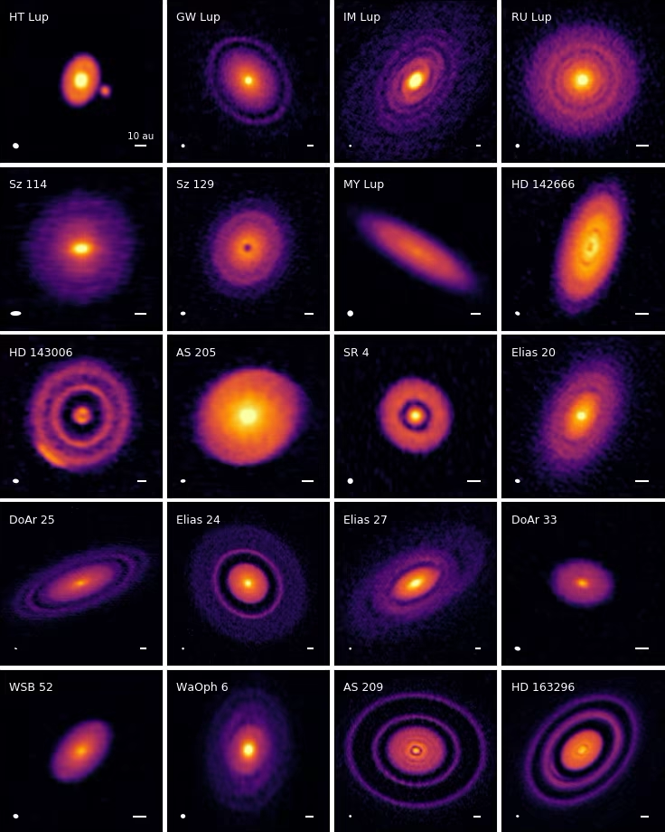
Fig. 14.4 Gallery of 240 GHz (1.25 mm) ALMA continuum images of 20 nearby protoplanetary disks from the DSHARP large programme. Concentric rings, gaps, and asymmetric features are nearly ubiquitous, and most are interpreted as signatures of planetary growth in progress. The combination of disk substructure surveys with disk dust mass measurements provides the strongest empirical constraints on the inputs to planet formation models. Reproduced from Andrews et al. [2018].

Fig. 14.5 compares the core growth times of pebble and planetesimal accretion across the disk.

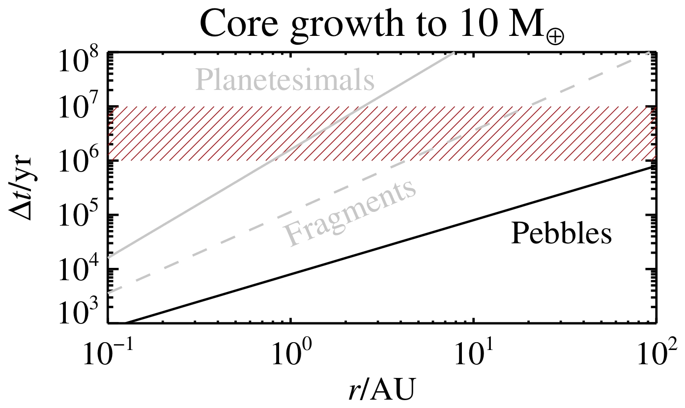
Fig. 14.5 Time required to grow a 10 Earth mass core as a function of distance from the star. The solid black line is pebble accretion in the Hill regime, the solid grey line is planetesimal accretion, and the dashed grey line is accretion of planetesimal fragments from a thin midplane layer. The red hatched band, roughly 1 to 10 Myr, is the interval over which the disk loses its gas, so a core that is to capture a gas envelope must reach 10 Earth masses before it. The pebble line stays below the band at every radius plotted, while the planetesimal line rises through it within a few AU and lies above it in the outer disk. Reproduced from Lambrechts and Johansen [2012].

Disk migration explains close-in giants and resonant chains, systems locked in near-integer period ratios (Lecture 13).

Jupiter’s early growth may have isolated the non-carbonaceous and carbonaceous (NC-CC) meteorite reservoirs [Kruijer et al., 2017] (Fig. 14.6).

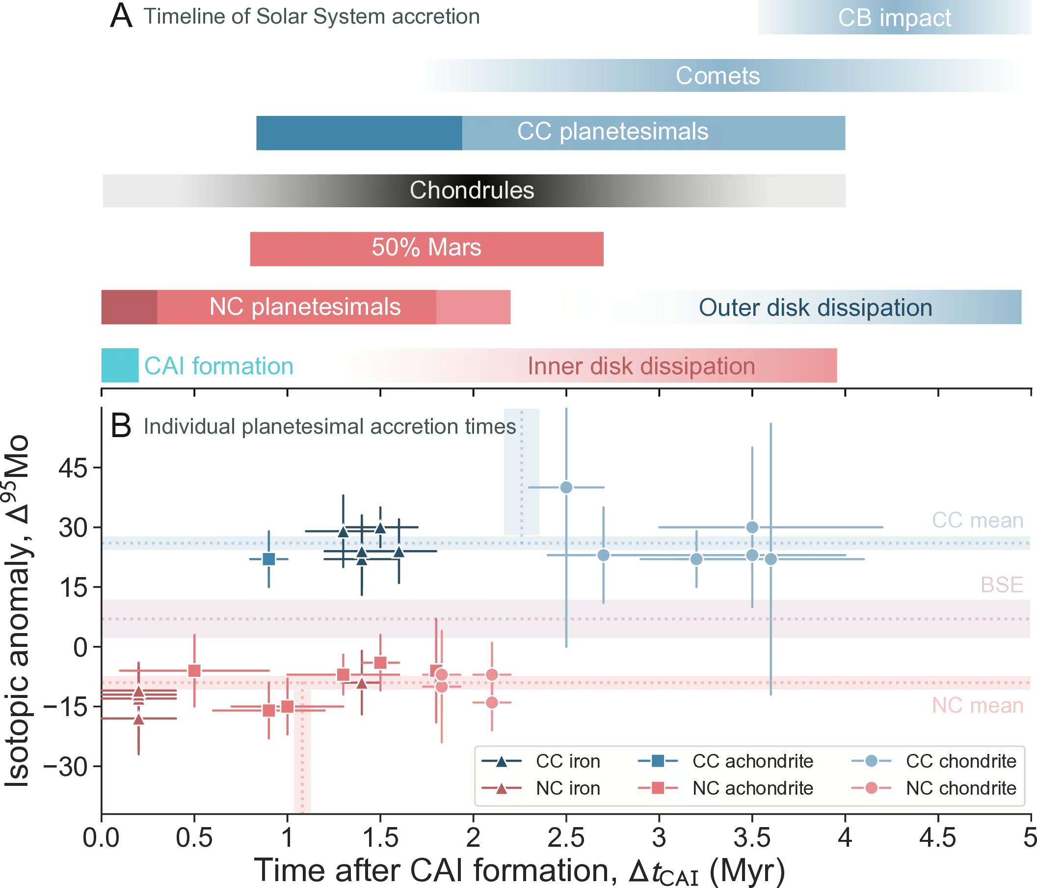
Fig. 14.6 Timeline of solar system formation reconstructed from isotopic dating of meteoritic materials. The non-carbonaceous (NC, red) and carbonaceous (CC, blue) reservoirs maintain distinct isotopic signatures from CAI (calcium-aluminium-rich inclusion, among the earliest solids to condense in the solar system) formation onwards, indicating that they accreted in physically separated regions of the disk for at least the first 2 to 3 Myr. Reproduced from Lichtenberg et al. [2023].

Surveys reveal a radius valley at \(\sim 1.8\,\Rearth\) separating super-Earths from sub-Neptunes [Fulton et al., 2017] (Fig. 14.7; Lecture 13). Photoevaporation by stellar XUV [Owen and Wu, 2017] and core-powered mass loss [Gupta and Schlichting, 2019] both predict a valley in the right location, and current data cannot yet reject either mechanism.

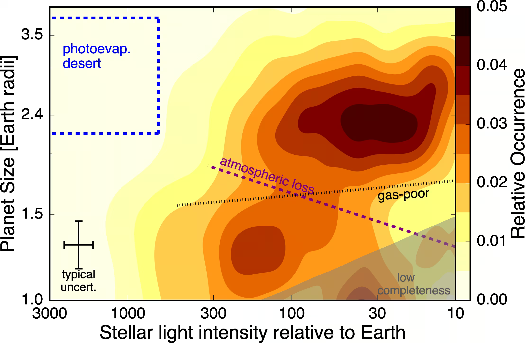
Fig. 14.7 The “Fulton gap” in the radius distribution of small close-in exoplanets. The two-dimensional map of planet size against incident stellar light shows a deficit of planets at \(\sim 1.8\,\Rearth\) that separates a denser super-Earth population from a sub-Neptune population. The dashed line marks the location of the valley predicted by atmospheric-loss (photoevaporation) models; the dotted line marks a gas-poor formation model. Reproduced from Fulton et al. [2017].

Meteorite reservoir separation may require Jupiter core growth within \(\sim 1\) Myr of CAIs [Kruijer et al., 2017]. Alternatively, the snow line, the disk radius where water ice condenses, divides reservoirs without an early core [Lichtenberg et al., 2021]. This is unresolved and matters for whether Jupiter set the boundary conditions of inner-system planet formation.

Planets between \(1\) and \(4\,\Rearth\) are the most common exoplanets [Fressin et al., 2013, Fulton et al., 2017], yet the solar system contains none. This absence may reflect pebble blocking by Jupiter, low solid density, or stochastic history.

Population synthesis models simulate planet formation to predict demographic outcomes (Fig. 14.8). Synthetic populations produce super-Earths, confirming that their absence in the solar system requires a specific dynamical explanation.

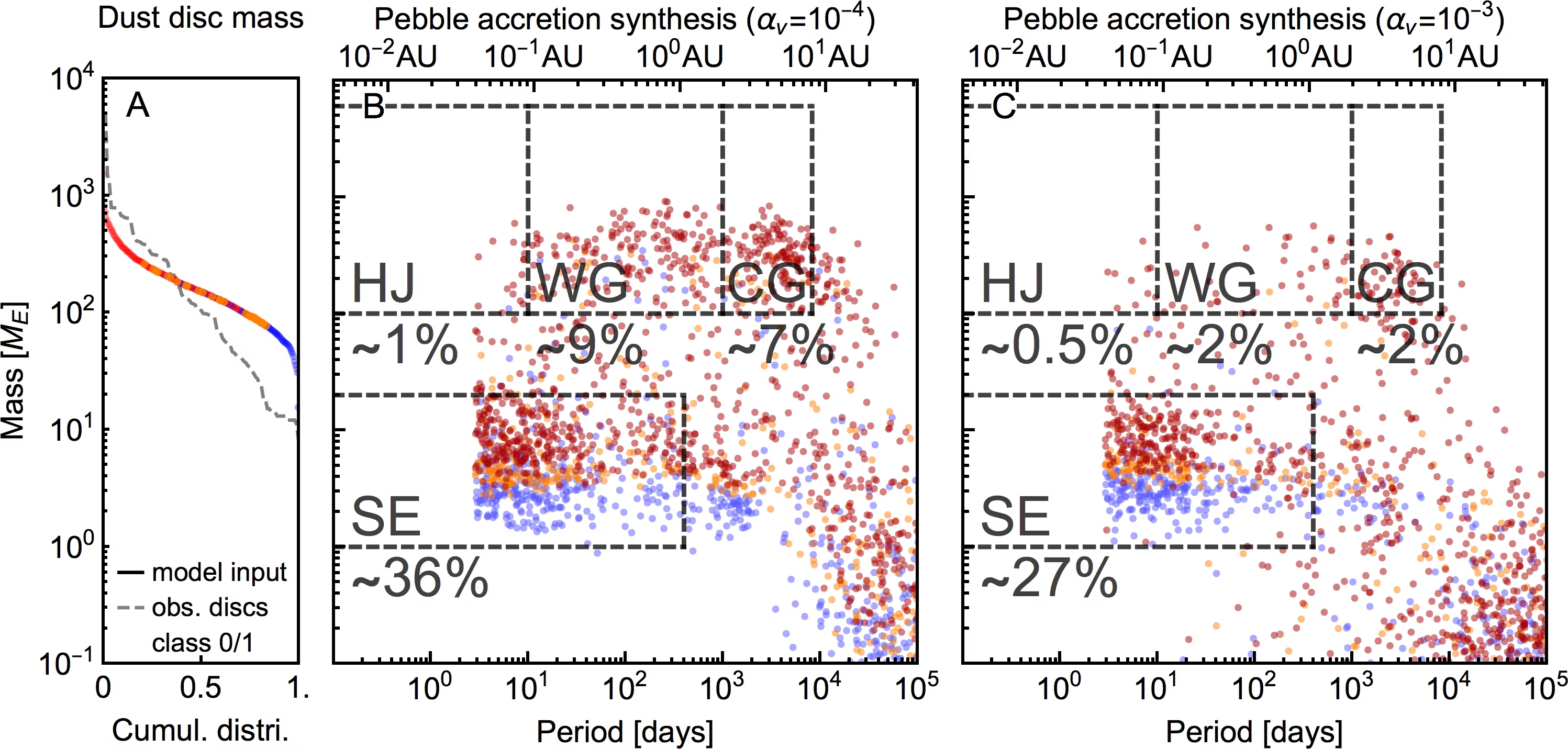
Fig. 14.8 Population synthesis predictions for planet mass versus orbital period from pebble accretion at low (panel B, \(\alpha_\nu = 10^{-4}\)) and moderate (panel C, \(\alpha_\nu = 10^{-3}\)) turbulence, drawn from the dust disc mass distribution of panel A. Both runs populate the super-Earth, hot Jupiter, warm gas giant, and cold gas giant regimes, with super-Earth fractions of \(\sim 36\%\) and \(\sim 27\%\). Reproduced from Drążkowska et al. [2023].

These results lead to one conclusion. Formation theory now explains how each observed type of planet, from super-Earths and sub-Neptunes to hot and cold giants, can form within the lifetime of the gas disk, and disk images show this process in progress. It cannot yet predict which type a given disk produces: population synthesis returns the full range of types from one set of physics, and the proportions change with poorly constrained inputs such as the disk turbulence (Fig. 14.8). The solar system is one outcome of this process, and two of its features are the test cases for the comparison that follows: a Jupiter that may have formed within about \(1\) Myr, and the absence of any planet between \(1\) and \(4\,\Rearth\).

14.1.3. The solar system overlaid on the exoplanet diagram

The period-radius diagram highlights where our solar system differs from exoplanet architectures (Lecture 13).

Fig. 14.9 shows the period-radius census with the compact multis marked.

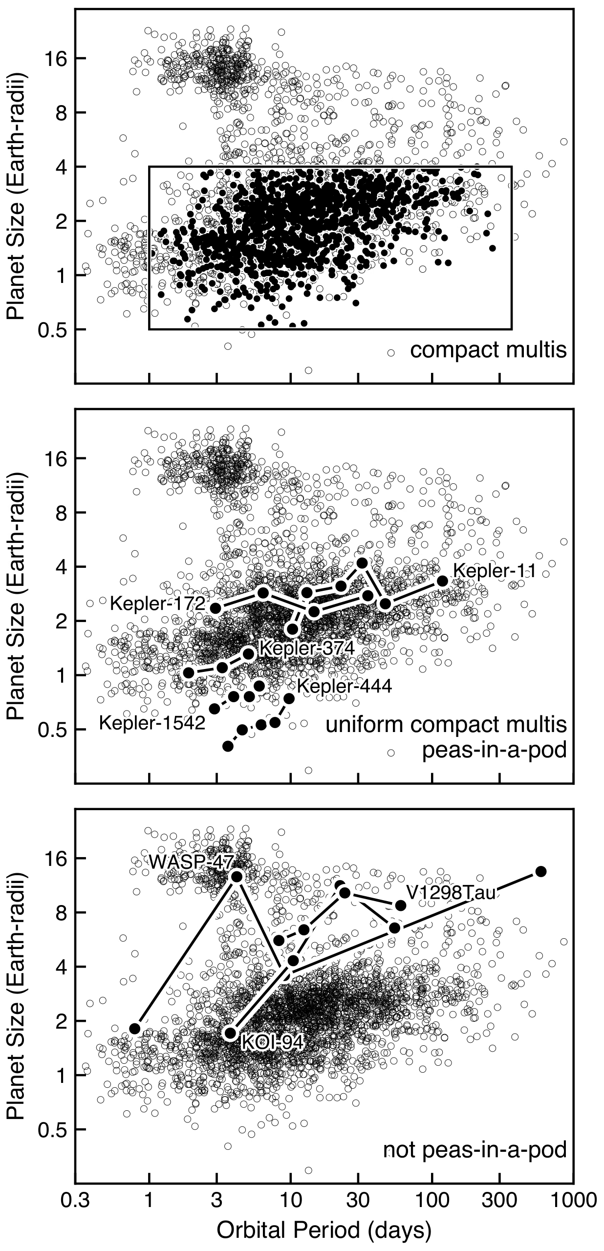
Fig. 14.9 Census of confirmed transiting exoplanets in orbital period and planet size. Open circles are all transiting planets. The box in the top panel is the region used to define a compact multi, a system with at least two planets inside it, and the filled circles are the planets that meet that definition. The middle panel joins the planets of five compact multis whose sizes and spacings are unusually uniform (Kepler-11, Kepler-172, Kepler-374, Kepler-444, Kepler-1542), the “peas-in-a-pod” pattern. The bottom panel joins three systems that do not show it: WASP-47 and KOI-94 meet the compact-multi definition but span a wide range of planet sizes, and the young system V1298 Tau fails it. Reproduced from Weiss et al. [2023].

A disk snow line creates a typical radial composition gradient [Weiss et al., 2023], but four features are unusual:

1. No planets between \(1\,\Rearth\) and \(\sim 4\,\Rearth\), though most stars host one within 1 AU [Bergsten et al., 2022].

2. Circular giant orbits at 5 and 10 AU rather than eccentric orbits.

3. No hot Jupiter, found around fewer than \(1\%\) of Sun-like stars (\(0.43\%\) for periods below 10 days; Fressin et al. [2013]), and no hot Neptune, which falls in the hot-Neptune desert [Mazeh et al., 2016].

4. Irregular terrestrial spacings rather than uniform peas-in-a-pod architectures (Fig. 14.10; Weiss et al. [2018]).

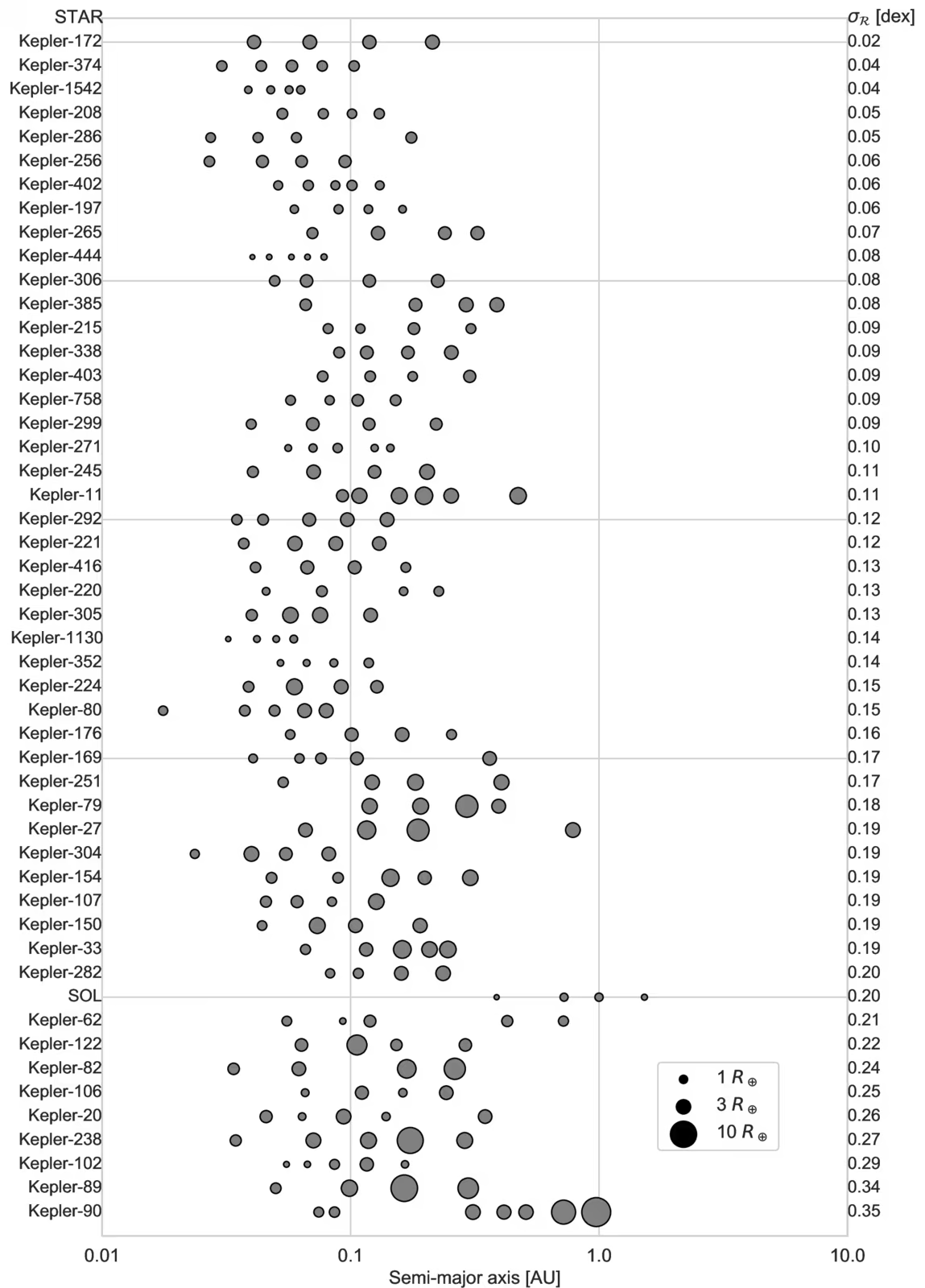
Fig. 14.10 Compact multi-planet systems with four or more transiting planets interior to 1.52 AU, ranked by their planet-radius dispersion (most uniform sizes at the top, greatest size diversity at the bottom). Point sizes scale logarithmically with planet radius. The solar system terrestrials, included for comparison, sit in the bottom quintile of size uniformity, showing that the peas-in-a-pod architecture prevalent in Kepler compact multis did not emerge in our own system. Reproduced from Weiss et al. [2023].

The mass-radius diagram evaluates bulk composition against theoretical equations of state (Fig. 14.11). Terrestrial planets follow the Earth-like rocky curve, while larger sub-Neptunes sit above it with volatile envelopes.

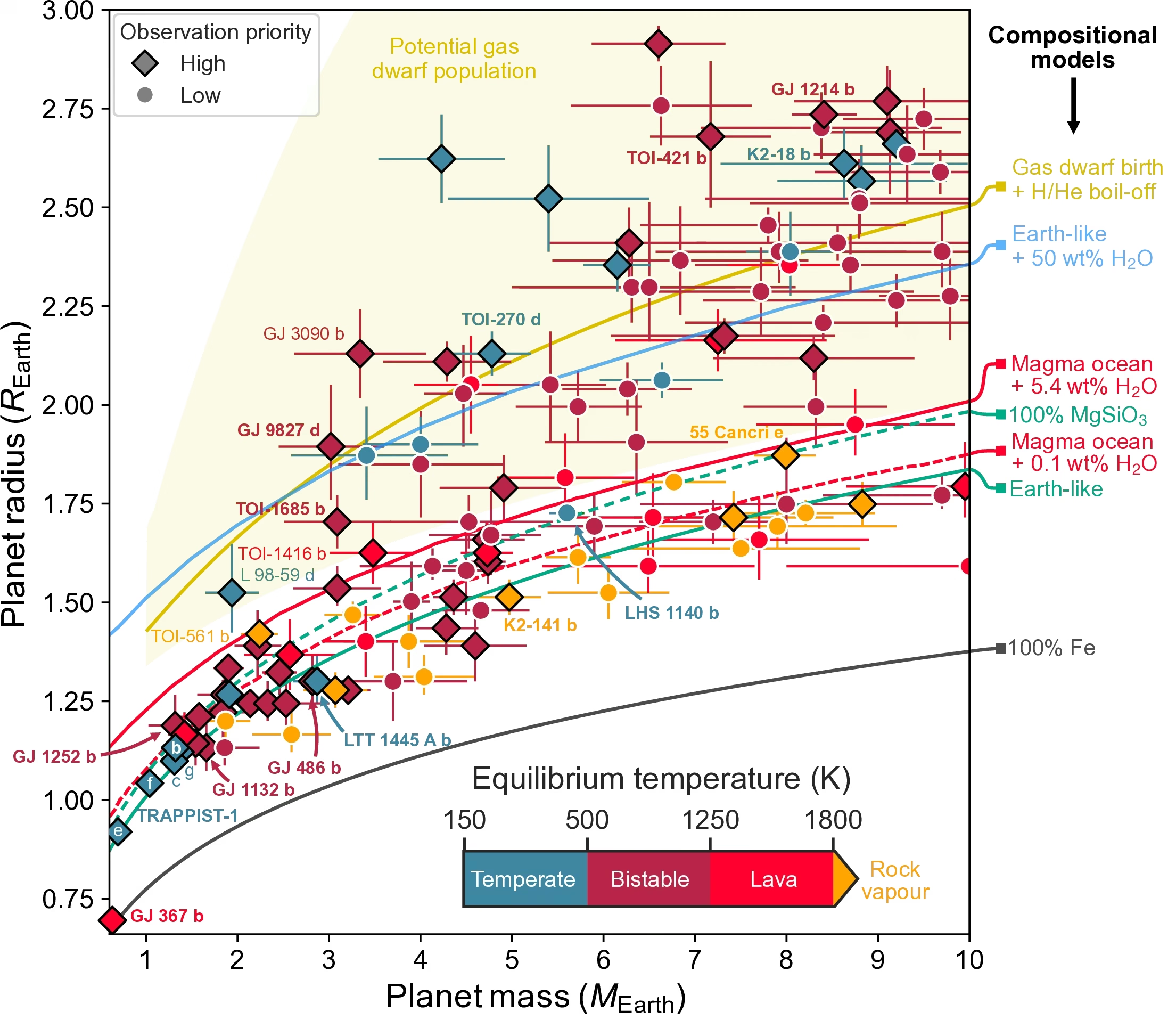
Fig. 14.11 Mass-radius diagram for rocky and small exoplanets from Lichtenberg et al. [2025] Fig. 2. Data points are observed exoplanets with measured masses and radii, colour-coded by equilibrium temperature into temperate (blue, 150 to 500 K), bistable (crimson, 500 to 1250 K, able to sit in either a temperate or a runaway-greenhouse climate state), lava (red, 1250 to 1800 K), and rock-vapour (orange, above 1800 K) regimes; symbol shape marks high-priority atmospheric-characterisation targets (diamonds) and lower-priority targets (circles). Labelled planets include TRAPPIST-1 b, c, e, f and g, GJ 367 b, GJ 1132 b, GJ 486 b, GJ 1252 b, GJ 1214 b, GJ 3090 b, GJ 9827 d, 55 Cancri e, K2-18 b, K2-141 b, LHS 1140 b, L 98-59 d, LTT 1445 A b, and several TOI targets. Theoretical equation-of-state tracks range from 100% Fe (bottom) through Earth-like rocky and 100% \(\mathrm{MgSiO_3}\), with volatile-rich tracks for Earth-like + 50 wt% \(\mathrm{H_2O}\), magma ocean + 0.1 wt% or 5.4 wt% \(\mathrm{H_2O}\), and a gas-dwarf birth + H/He boil-off curve that runs through the potential gas-dwarf population (shaded). Planets above the Earth-like curve either retain volatile envelopes (H/He, water, or melt-water mixtures) or are otherwise reshaped by magma-ocean outgassing and photoevaporation. Reproduced from Lichtenberg et al. [2025].

14.1.4. “Is the solar system rare?”

Whether the solar system is rare remains unknown because survey limits have left much of its parameter space unobserved. Detecting a planet in a 12-year Jupiter-like orbit requires a baseline of a decade or more: long-term radial-velocity surveys find such planets around nearby stars, and Gaia astrometry will add them at scale, with DR4 (5.5 years of data, planned for December 2026) covering part of such an orbit and DR5 (the full mission, not before 2030) a complete one. Earth analogues (\(\Rearth\)-sized planets in 1-year orbits around Sun-like G dwarfs) lie beyond current sensitivity. Their astrometric signal is far too small for Gaia (about \(0.3\,\mu\)as for an Earth at 1 AU around a Sun-like star 10 pc away), so they require transit surveys such as PLATO (launch planned for 2027) and, later, direct imaging with HWO or LIFE.

The planet occurrence rate (the average number of planets per star in a given parameter range) depends strongly on stellar type (Fig. 14.12). Rocky and sub-Neptune-sized planets on orbits with periods \(< 50\) days are two to four times as common around early M dwarfs as around F, G and K dwarfs, although whether this reflects formation efficiency or survey detection bias remains debated.

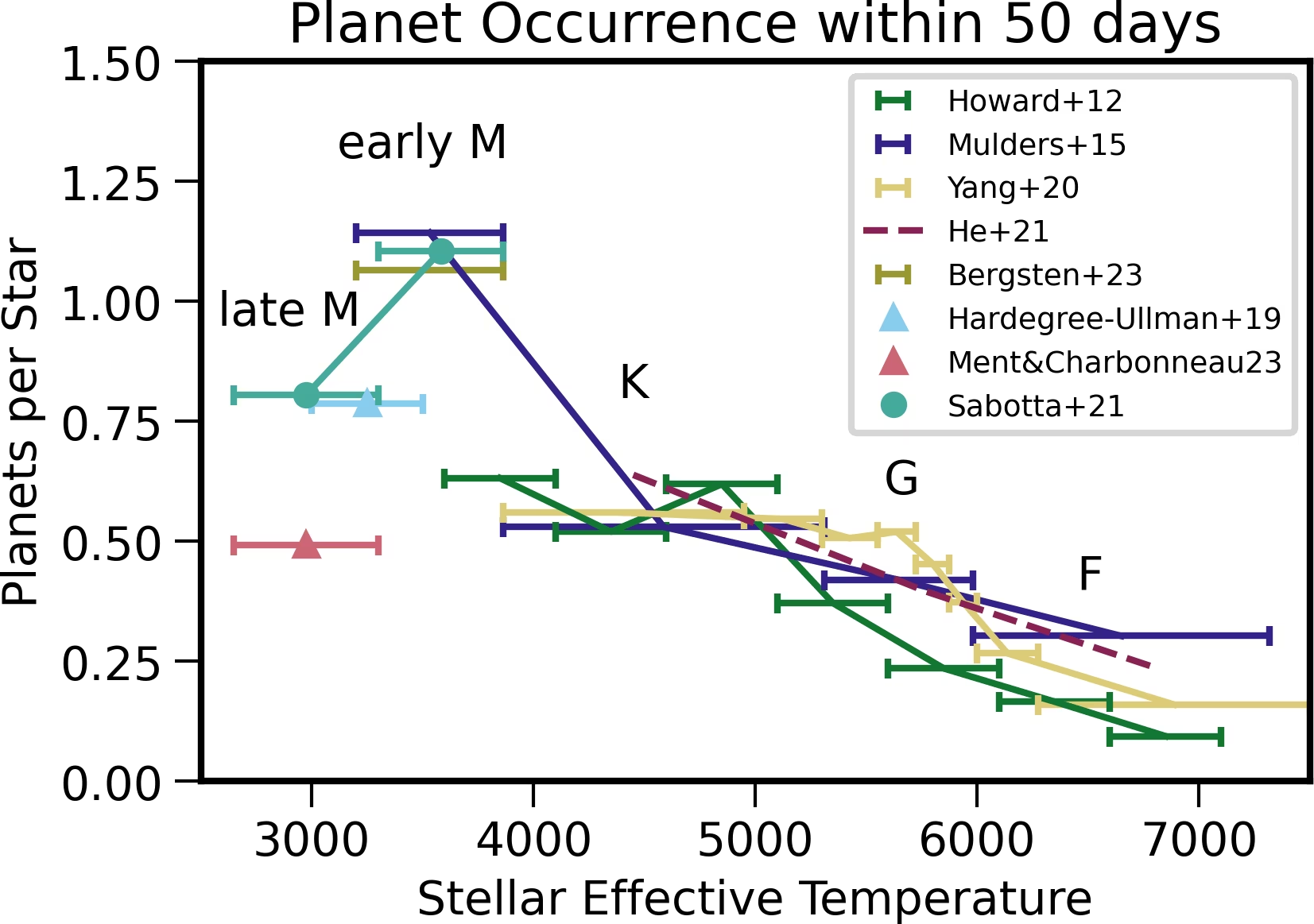
Fig. 14.12 Overview of planet occurrence rates as a function of host-star effective temperature, for planets between \(1\) and \(4\,\Rearth\) on orbital periods \(P < 50\) days, from Mulders [2024] Fig. 5. Rates were re-scaled assuming uniform occurrence in \(\log P\) and \(\log R\) for cross-study comparison. Plotted data are compiled from Howard+12, Mulders+15, Hardegree-Ullman+19, Yang+20, He+21, Sabotta+21, Bergsten+23, and Ment & Charbonneau 23 (see Mulders [2024] for full references). Across all studies, planet occurrence increases from F dwarfs (\(\sim 6500\) K) to early M dwarfs (\(\sim 3500\) K), where it is a factor of \(\sim 2\) to 4 higher than around FGK stars; a break appears toward late M dwarfs, but those surveys sample only very short periods (\(< 10\) d), so the late-M values are potentially lower limits. The headline message is that small, close-in planets are most common around the most numerous class of stars in the galaxy. Reproduced from Mulders [2024].

14.2. Part 2: Habitability as a coupled systems property

14.2.1. The stack of requirements

Habitability is the capacity of a planet to sustain surface liquid water, which emerges from a stack of coupled physical requirements rather than a single condition. Earlier lectures developed these components in sequence: atmospheric retention in lecture 5, climate feedbacks in lecture 6, tectonics in lecture 7, comparative evolution of Earth, Venus, and Mars in lectures 9 and 10, and stellar context in lecture 13.

The stack spans requirements across the planetary system:

• Star: Stable luminosity over Gyr timescales, low flaring, and a long main-sequence lifetime.

• Orbit: Location in the liquid-water habitable zone, low eccentricity, and heat redistribution preventing atmospheric collapse.

• Planet bulk: Sufficient mass to retain volatiles over Gyr timescales and drive mantle convection.

• Atmosphere: Composition maintaining temperate conditions without runaway photochemistry.

• Interior: Internal heat driving mantle convection, outgassing, and dynamo generation.

• Surface and tectonics: Volatile recycling between the surface, atmosphere, and interior must close the carbon cycle.

• Biosphere: Biological feedbacks modifying atmospheric composition, surface albedo, and weathering.

Every level in the stack is necessary, but none is sufficient alone. Habitability is a system property governed by coupled feedbacks. Stellar radiation drives photochemistry, clouds affect albedo and temperature, temperature regulates weathering that draws down \(\mathrm{CO_2}\), and outgassing replenishes \(\mathrm{CO_2}\) through tectonic recycling. Breaking any coupling can drift the climate into a state where surface liquid water cannot persist.

Fig. 14.13, from Meadows and Barnes [2018], organizes these habitability factors into stellar, planetary-system, and planetary properties. The diagram distinguishes properties by accessibility: direct observations, model interpretations, or theoretical constraints. This distinction determines which couplings telescopes can actually test.

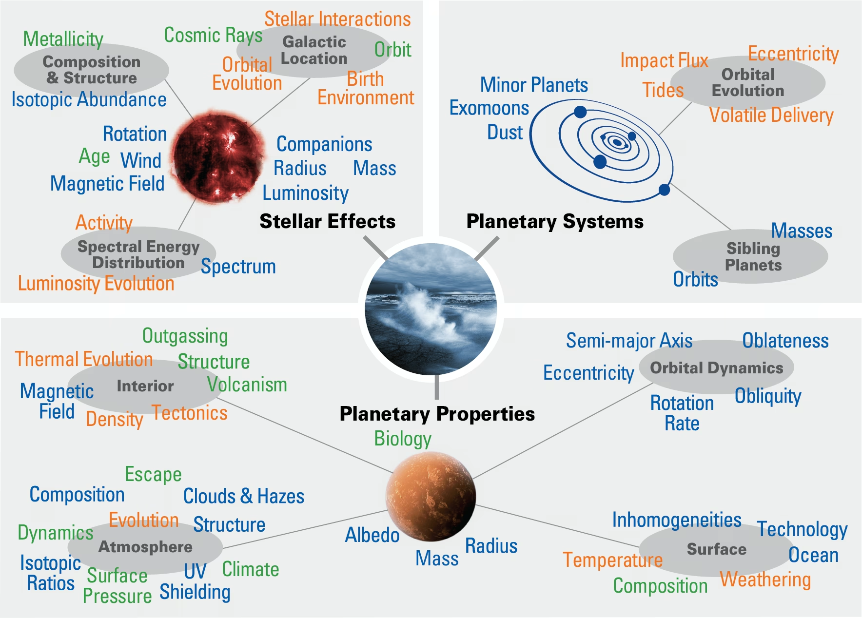
Fig. 14.13 Factors affecting planetary habitability: the currently understood stellar, planetary-system, and planetary properties that may impact whether a planet can sustain surface liquid water. Font colour denotes how each characteristic is accessible: blue for properties that could be observed directly with sufficiently powerful telescopes, green for those that require modelling interpretation, possibly constrained by observations, and orange for properties or processes accessible primarily through theoretical modelling. The larger the number of these factors that can be determined for a habitable zone candidate, the more robust the assessment of its habitability. Reproduced from Meadows and Barnes [2018].

14.2.2. The habitability coupling loop

On a tidally locked planet, rotation and orbital periods match so that one hemisphere permanently faces the star (Fig. 14.14; Wordsworth and Kreidberg [2022]). Substellar clouds reflect starlight, super-rotating winds transport heat to the nightside, and antistellar cold-trapping can collapse the atmosphere.

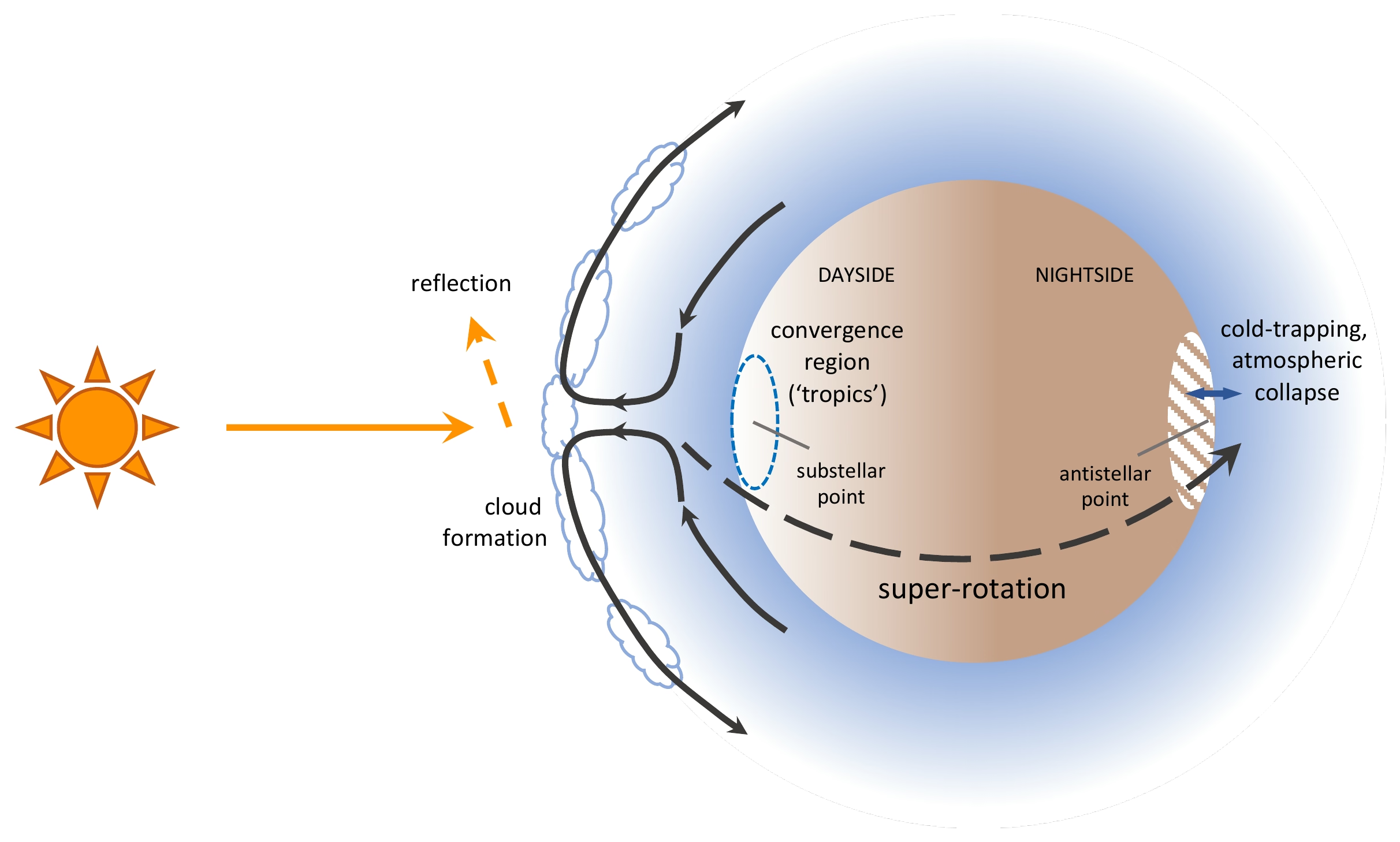
Fig. 14.14 Schematic of the dynamical and climate processes in the atmosphere of a tidally locked rocky exoplanet. Stellar irradiation drives cloud formation and partial reflection near the substellar point, day-to-night heat transport by super-rotating winds, and cold-trapping of condensable volatiles at the antistellar point, where the atmosphere can collapse onto the surface. When the dominant condensable is water, this transport-and-trapping cycle is the planet’s hydrological cycle. Whether it persists depends on the total water inventory and on factors such as tectonic regime, escape, and stellar evolution that this single snapshot does not capture. Reproduced from Wordsworth and Kreidberg [2022].

The full coupling loop links the star, atmosphere, surface, and interior. Stellar irradiation drives radiative balance and photochemistry (Lecture 5), while atmospheric heating controls surface weathering and carbonate-silicate breakdown (Lecture 6, Lecture 9). Subduction returns volatiles to the deep mantle, interior outgassing supplies \(\mathrm{CO_2}\), \(\mathrm{H_2O}\), and \(\mathrm{SO_2}\), and dynamo shielding deflects the stellar wind (Lecture 4).

Neither equilibrium temperature nor habitable zone position alone determines habitability. A planet remains habitable only if all coupling loops remain closed across geological history under appropriate boundary conditions.

14.2.3. The habitable zone is not a line

The habitable zone (HZ) is the orbital range around a star where an Earth-like planet can maintain liquid surface water. Its boundaries are set by the runaway greenhouse limit and maximum \(\mathrm{CO_2}\) greenhouse [Kopparapu et al., 2013] (Fig. 14.15).

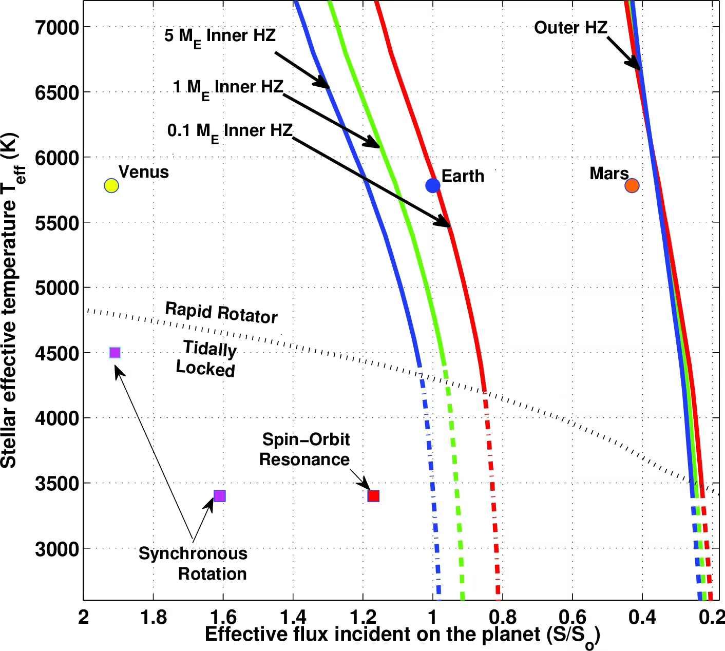
Fig. 14.15 Habitable zone boundaries as a function of stellar effective temperature and planet mass, from Kopparapu et al. [2014]. The inner HZ (left curves) and outer HZ (right curve) shift inward for cooler stars. Around M dwarfs, the HZ overlaps strongly with the tidal-locking radius and with spin-orbit resonance regions, where the planet’s rotation period locks to a simple ratio of its orbital period, complicating habitability assessment in ways that the 1D HZ does not capture. Reproduced from Kopparapu et al. [2014].

Venus receives \(\sim 1.9\times\) Earth’s solar flux but has a \(737\) K, \(92\) bar atmosphere without water, while Earth maintains a \(288\) K surface and stable hydrosphere (Lecture 9). This divergence reflects different histories through early molten phases and solar luminosity evolution [Hamano et al., 2013] (Fig. 14.16).

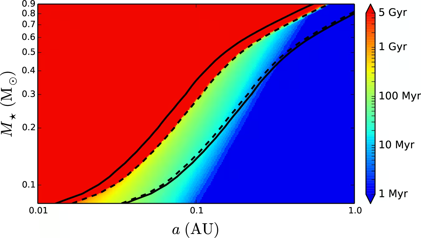
Fig. 14.16 Duration of the runaway greenhouse phase for planets that formed at 10 Myr with abundant surface water, as a function of stellar mass (vertical axis) and orbital semi-major axis (horizontal axis), from the Luger and Barnes [2015] water-loss calculation around M dwarfs. The solid black lines mark the empirical habitable zone, from the recent-Venus limit (left) to the early-Mars limit (right); the dashed lines mark the theoretical runaway greenhouse (left) and maximum greenhouse (right) limits; all limits are for a stellar age of 5 Gyr. Habitable-zone planets around late M dwarfs spend a substantial fraction of their first Gyr inside the runaway state, losing much of their initial water before the host star reaches the main sequence. Reproduced from Luger and Barnes [2015].

The habitable zone is also time-dependent, as stellar luminosity rises along the main sequence: the Sun is about 30% brighter today than when it formed. Around M dwarfs, planets now in the HZ spent hundreds of Myr inside the runaway greenhouse boundary [Luger and Barnes, 2015].

The outer edge is uncertain for a different reason. The maximum \(\mathrm{CO_2}\) greenhouse limit leaves out \(\mathrm{CO_2}\) ice clouds, whose net warming is now thought to be small except around hot stars [Kitzmann, 2017]. Three-dimensional models show that on a frozen planet \(\mathrm{CO_2}\) condenses into permanent polar ice caps, so an Earth-like planet beyond about \(1.27\) AU from a Sun-like star may never escape global glaciation [Turbet et al., 2017] (Lecture 13).

Habitability therefore depends on evolutionary trajectories, requiring coupled climate-evolution models rather than static 1D HZ boundaries.

14.2.4. Tectonic regime and the long-term thermostat

The carbonate-silicate cycle is Earth’s long-term thermostat by balancing volcanic \(\mathrm{CO_2}\) outgassing with silicate weathering and carbonate subduction (Lecture 6, Lecture 9). Warmer surface temperatures increase weathering rates, accelerating \(\mathrm{CO_2}\) removal and cooling the planet (Fig. 14.17). On a body whose stagnant lid has cooled the interior (Mars after \(\sim 1\) Ga), volcanic outgassing ceases and the thermostat loses its return path (Lecture 7, Lecture 10).

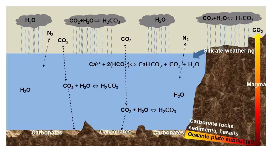
Fig. 14.17 Cartoon of the carbonate-silicate cycle on a planet with active plate tectonics. Atmospheric \(\mathrm{CO_2}\) dissolves in rainwater to form weak carbonic acid, which weathers continental silicates into bicarbonate ions; rivers transport these to the ocean, where they are precipitated as carbonate rocks; subduction then returns the carbon to the mantle. Volcanism completes the cycle by outgassing fresh \(\mathrm{CO_2}\). On geological timescales (of order \(0.5\) Myr), this cycle stabilises the surface temperature against perturbations. Reproduced from Lammer et al. [2018].

This thermostat requires liquid water, active volcanism, and plate tectonic recycling. Venus illustrates the failure of this mechanism (Lecture 9). Without liquid water, silicate weathering ceases, allowing outgassed \(\mathrm{CO_2}\) to accumulate into its 92 bar atmosphere. Stagnant-lid worlds (planets whose outer shell forms a single immobile plate rather than being recycled by plate tectonics) do not subduct carbonates into the mantle.

Whether stagnant-lid planets with episodic resurfacing can sustain temperate climates over Gyr timescales remains unresolved. Because planetary tectonic regimes cannot be measured remotely with current or near-term observations, this is one of the largest missing variables in assessing exoplanet habitability.

14.2.5. Magnetic field as gatekeeper

Lecture 4 and Lecture 10 showed how an active magnetosphere, a planetary magnetic shield, protects an atmosphere from solar-wind ion-pickup escape; Fig. 14.18 shows the shape of that shield for Earth.

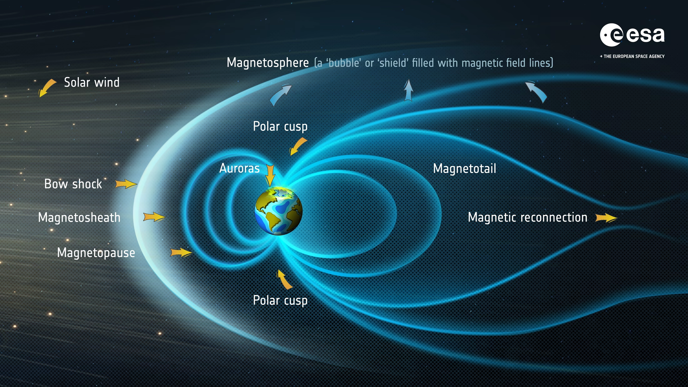
Fig. 14.18 Anatomy of Earth’s magnetosphere. The solar wind (orange arrows, arriving from the left) is slowed and deflected at the bow shock, and the shocked plasma flows around the planet through the turbulent magnetosheath. The magnetopause is the surface where the solar wind ram pressure is balanced by the magnetic pressure of Earth’s field; under typical conditions it lies at the standoff distance \(r_{\mathrm{mp}} \approx 10\,\Rearth\). Inside it, the dayside field is compressed, while the nightside field is stretched into the long magnetotail. Credit: ESA, CC BY-SA 3.0 IGO.

Mars lost its global magnetic field early in its history, with remanent magnetization indicating dynamo activity until \(\sim 3.7\) Ga near the Noachian-Hesperian boundary, later than the 4.1 to 3.9 Ga estimated from basin demagnetisation [Acuña et al., 1999, Mittelholz et al., 2020]. Mars subsequently lost most of its atmosphere to space, consistent with MAVEN constraints indicating an initially thicker \(\mathrm{CO_2}\) atmosphere [Jakosky et al., 2018].

However, a magnetic field is not strictly required for atmospheric retention, as Venus retains its \(\sim 92\) bar atmosphere without one. A magnetic field instead shifts the balance of escape mechanisms. Without one, atmospheric losses are dominated by nonthermal escape: pickup ions, sputtering, and ionospheric outflow. Whether these losses matter on Gyr timescales depends on planetary mass, the atmospheric column, stellar wind strength, and dynamo timing. For exoplanets around active M dwarfs like TRAPPIST-1, whether an active dynamo is required for atmospheric retention remains an open question.

14.2.6. Water delivery and planetary evolution

Planetary water inventories are often framed around delivery from carbonaceous chondrites (primitive, volatile-rich meteorites) versus comets and their relative D/H ratios. However, internal planetary evolution dominates over initial delivery in setting inner solar system water budgets.

Earth, Venus, and Mars accreted broadly similar volatile inventories per unit silicate mass [Lichtenberg et al., 2023]. Their present-day water inventories differ by orders of magnitude because each planet processed its initial inventory differently [Hamano et al., 2013].

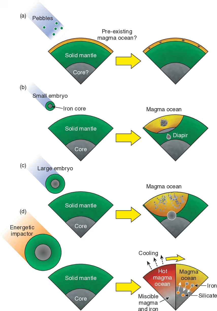
Fig. 14.19 Physical mechanisms of metal-silicate differentiation on a forming rocky planet, from Lichtenberg et al. [2023] Fig. 2. (a) Accreted pebbles may not melt a Mars-sized protoplanet but mix into a magma ocean if one is already present. (b) A small embryo melts a local magma pond in which its iron core breaks up; the metal settles and sinks through the solid mantle as a diapir. (c) A large embryo melts a large region, and its core sinks with little mixing. (d) An energetic impact can heat the interior until silicate and iron become miscible; they separate again as the magma ocean cools. How much of the mantle melts sets the conditions under which water and carbon partition between core, mantle and atmosphere (see text). Reproduced from Lichtenberg et al. [2023].

The first mechanism is volatile partitioning during the early molten phase, when the mantle is wholly or largely molten (a magma ocean). Water and carbon partition between the core, mantle, and overlying steam atmosphere according to magma redox state, solidification timescale, and crystallisation depth [Hirschmann, 2012], and how much of the mantle melts depends on how the planet accretes (Fig. 14.19). Different boundary conditions produce divergent atmospheric end states from identical initial budgets.

Accretion timing also controls volatile retention. Planetesimals accreting within the first \(\sim 1\) Myr after CAI formation are heated above the water-ice melting point by short-lived radionuclides (\(^{26}\mathrm{Al}\), half-life \(\sim 0.7\) Myr) and lose water by dehydration. Bodies accreting later beyond the snow line retain their volatiles [Lichtenberg et al., 2023].

The second mechanism is atmospheric escape during the magma ocean phase, where, on planets inside the runaway threshold (Type II of Hamano et al. [2013]), hydrodynamic escape removes the water before the surface solidifies (Fig. 14.20; Lecture 9).

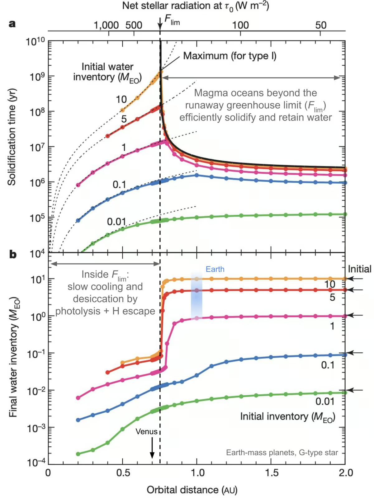
Fig. 14.20 Two distinct types of terrestrial planet defined by the Hamano et al. [2013] model. Panel (a) shows magma-ocean solidification time as a function of orbital distance and instellation for a range of initial water inventories; planets inside a critical orbital distance (\(\sim 0.76\) AU around a Sun-like star) cannot solidify their magma oceans before most of their water is lost to hydrodynamic escape (“Type II”), while planets further out solidify quickly and retain most of their water (“Type I”). Panel (b) shows the resulting final water inventories at the end of magma-ocean solidification. Modified from Hamano et al. [2013] as reproduced in Lichtenberg et al. [2023].

The third mechanism is long-term mantle-atmosphere volatile exchange. On planets with active plate tectonics, outgassing and subduction balance to maintain steady surface inventories over billions of years.

The fourth mechanism is stellar evolution. For M-dwarf planets, the luminous pre-main-sequence phase keeps the habitable zone within the runaway greenhouse boundary for the first few hundred Myr (Lecture 13; Luger and Barnes [2015]).

Radiogenic clocks in meteorites and lunar samples show that core formation, magma ocean crystallisation, and silicate differentiation finished within the first \(\sim 100\) Myr [Lichtenberg et al., 2023].

The D/H ratios from Lecture 12 constrain delivery combined with evolutionary processing. Likewise, exoplanet atmospheric water observations reflect the integrated history of accretion, magma-ocean processing, escape, outgassing, and tectonic recycling.

14.2.7. The Drake equation and its limitations

The Drake equation is a heuristic factorisation organising questions about communicating civilisations in the galaxy, written for the 1961 Green Bank meeting [Drake, 1965]:

\[ N = R_\star \cdot f_p \cdot n_e \cdot f_l \cdot f_i \cdot f_c \cdot L \,. \]

Here \(R_\star\) is the galactic star formation rate, \(f_p\) the fraction of stars with planets, \(n_e\) the number of habitable-zone planets per system, \(f_l\) the fraction hosting life, \(f_i\) the fraction evolving intelligence, \(f_c\) the fraction developing broadcasting technology, and \(L\) the communicative lifetime.

Stellar astrophysics determines \(R_\star\), while exoplanet surveys show that \(f_p\) is of order unity (Lecture 13). For Sun-like stars, Kepler data give \(n_e\) between about \(0.4\) and \(0.9\) rocky planets per star in the habitable zone, depending on the habitable-zone definition and on how the survey completeness is extrapolated to long orbital periods, with large uncertainties [Bryson et al., 2021]. In contrast, Earth provides the sole data point for \(f_l\), whereas \(f_i\), \(f_c\), and \(L\) have no statistical constraints beyond our own lineage and the last \(\sim 100\) years.

The Drake equation is a qualitative framework rather than a predictive estimator, because point estimates of \(N\) face five fundamental limitations:

1. Coupled factors: biospheres co-evolve with planetary interiors and atmospheres, preventing strict factor independence.

2. Orders-of-magnitude uncertainty: published estimates for \(f_l\), \(f_i\), \(f_c\), and \(L\) span four to ten orders of magnitude, reflecting input priors rather than data.

3. Non-equilibrium contingency: the origin of life is a historical, non-equilibrium process rather than a stationary Markov chain.

4. Assumed uniformity: the single-parameter formulation averages across diverse stellar environments, planet types, and evolutionary histories.

5. Anthropic selection: Earth is our only observed example of life, creating an observer selection effect.

Sampling each factor across published ranges (Fig. 14.21), Sandberg et al. [2018] found in their resampling of the published ranges that about one third of the probability falls at \(N < 1\): no other civilisation in the Milky Way. About ten percent falls at \(N < 10^{-10}\): no other civilisation in the observable universe. Sandberg et al. [2018] argue that this dissolves the Fermi paradox, the apparent contradiction between high estimates of extraterrestrial civilisations and the lack of observational evidence.

Because unconstrained factors spanning multiple decades require log-uniform priors, taking the logarithm converts the product into a sum:

\[ \log_{10} N = \log_{10}(R_\star f_p n_e) + \log_{10} f_l + \log_{10} f_i + \log_{10} f_c + \log_{10} L \,, \]

Each of the four unconstrained terms can span ten or more decades: the fractions \(f_l\), \(f_i\) and \(f_c\) anywhere between \(10^{-10}\) and 1, and the lifetime \(L\) over many decades of years. Their sum, and with it the distribution of \(N\) obtained by sampling the factors, therefore spreads over tens of decades.

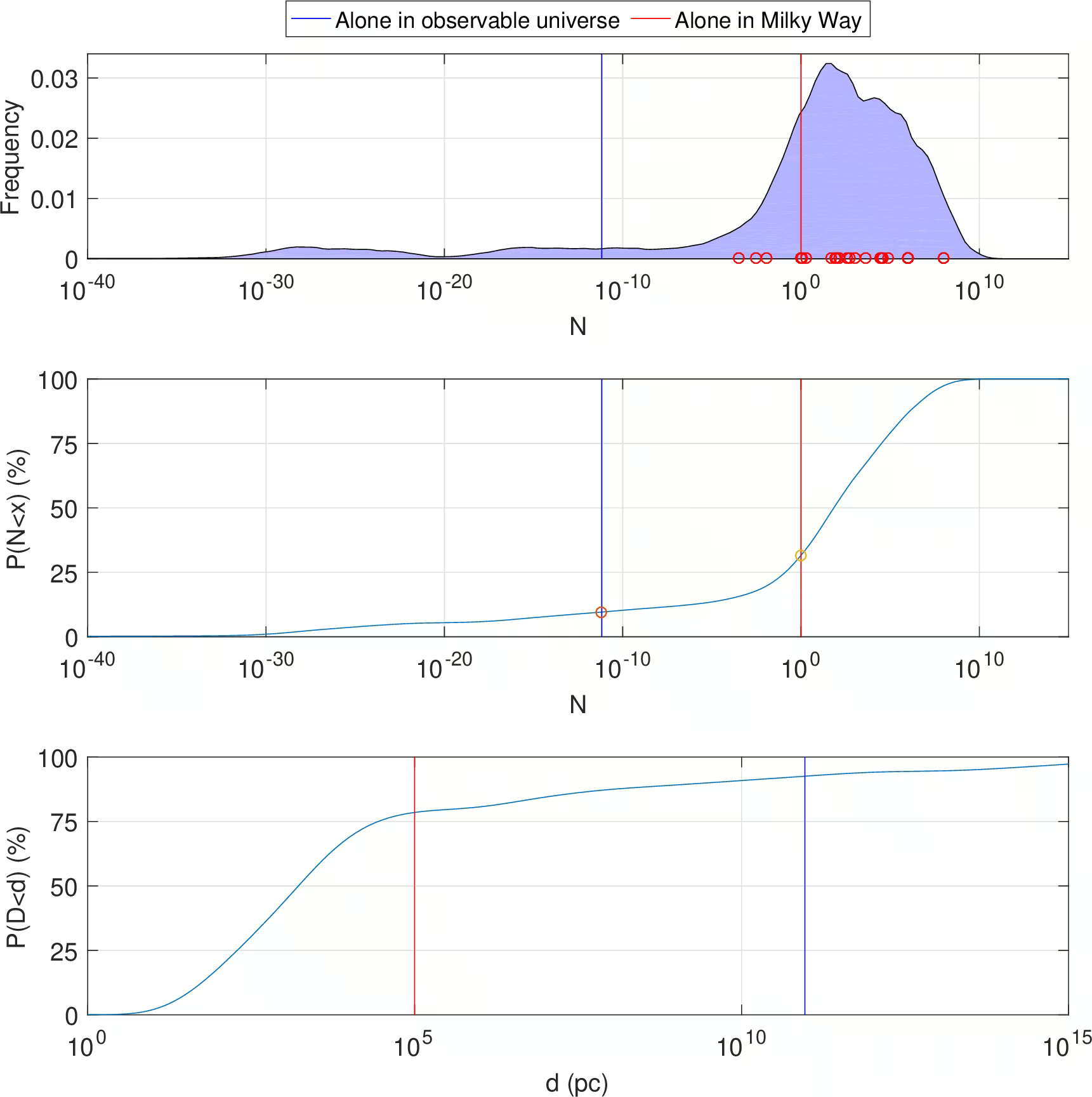
Fig. 14.21 Distribution of the number \(N\) of communicating civilisations in the Milky Way from Monte-Carlo sampling across published parameter ranges (top), its cumulative form (middle), and the implied distance to the nearest civilisation (bottom) [Sandberg et al., 2018]. The red line marks \(N = 1\) (no other civilisation in the Milky Way) and the blue line \(N = 10^{-10}\) (none in the observable universe). About one third of the probability lies below the first line and ten percent below the second.

14.2.8. The Fermi paradox

The Fermi paradox is the question of why we observe no evidence of spacefaring civilisations, summarised as “where is everybody?”. Because the Milky Way is about \(10^{10}\) years old, an early spacefaring civilisation could have crossed the galaxy at sub-relativistic speeds. Yet, we observe no evidence of any such civilisation.

Proposed resolutions address different Drake-equation factors or observational limits:

• Rare-life hypothesis: \(f_l\) is very small because life is hard to start.

• Rare-intelligence hypothesis: \(f_i\) is the bottleneck because technological intelligence rarely follows from biology.

• Great filter: \(L\) is short because civilisations self-terminate before covering the galaxy.

• Detection threshold: signals exist but remain below current sensitivity or use unrecognised encoding.

• Zoo scenarios: civilisations deliberately conceal themselves or avoid contact.

The Fermi paradox is a tool for thinking rather than a piece of evidence. It is a check on intuition for Drake-equation estimates. An estimate of \(N \sim 10^4\) requires a mechanism that keeps civilisations invisible. An estimate of \(N \sim 1\) dissolves the paradox but raises the question of why life is so rare.

Fig. 14.22 places the resolutions on the Drake chain and states the timescale mismatch behind the paradox.

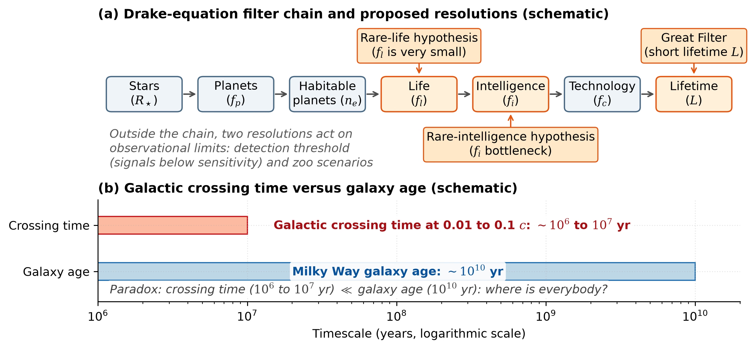
Fig. 14.22 The Fermi paradox as a chain of filters. (a) The Drake-equation factors as a sequence from stars to the lifetime of a technological civilisation. The three resolutions that act on single factors are the rare-life hypothesis (small \(f_l\)), the rare-intelligence hypothesis (\(f_i\) as the bottleneck) and the Great Filter (short \(L\)); the detection-threshold and zoo resolutions act on observational limits instead. (b) The timescale mismatch: across a Galaxy about \(10^5\) light years wide, a civilisation travelling at 0.01 to 0.1 \(c\) needs \(10^6\) to \(10^7\) yr, three to four orders of magnitude less than the \(10^{10}\) yr age of the Milky Way. Course-original figure.

14.3. Blackboard derivation: The habitable zone boundaries

Blackboard derivation: The habitable zone boundaries

The aim of this derivation is to reconstruct the inner and outer edges of the classical habitable zone from a one-line energy balance. The inputs are the inverse-square law, the Stefan-Boltzmann law and two flux limits from 1D radiative-convective climate models; the outputs are the orbital distances at which an Earth-like planet around a star of luminosity \(L_\star\) can support liquid surface water. After deriving the result in general, we will compare HZ widths for G, K, and M dwarfs.

Setup. A star of bolometric luminosity \(L_\star\) irradiates a planet at orbital distance \(d\). The flux at the planet’s orbit is

\[ F_\star(d) = \frac{L_\star}{4\pi d^2}\,. \]

Step 1: Equilibrium temperature. The planet absorbs a fraction \((1 - A_B)\) of the incident flux, where \(A_B\) is the Bond albedo. For a fast-rotating spherical planet, the absorbed power per unit area, averaged over the whole planet, is \((1 - A_B) F_\star / 4\), because the projected area is \(\pi R_p^2\) but the radiating area is \(4\pi R_p^2\). Equating absorbed and emitted power gives the equilibrium temperature

\[ T_{\mathrm{eq}}(d) = \left[\frac{L_\star (1 - A_B)}{16\pi\sigma\epsilon d^2}\right]^{1/4}\,, \]

where \(\epsilon\) is the effective emissivity of the atmosphere (which in the bare-rock limit is \(1\)) and \(\sigma\) is the Stefan-Boltzmann constant. For Earth around the Sun, plugging in \(A_B \approx 0.3\), \(\epsilon \approx 1\), \(L_\star = \Lsun\), and \(d = 1\) AU gives \(T_{\mathrm{eq}} \approx 255\) K. The actual surface temperature is \(\sim 288\) K because the greenhouse effect adds \(\sim 33\) K.

Fig. 14.23 shows the setup: the star of luminosity \(L_\star\), the planet at distance \(d\), and the habitable-zone strip between \(d_{\mathrm{in}}\) and \(d_{\mathrm{out}}\) that the derivation locates.

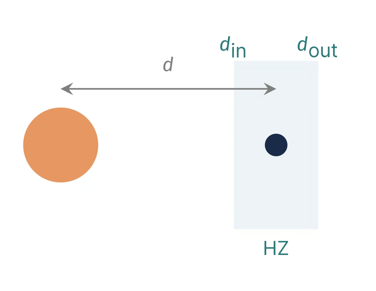
Fig. 14.23 Setup sketch of the board derivation of the habitable zone boundaries: a star of luminosity \(L_\star\), a planet at orbital distance \(d\), and the habitable zone (HZ) as the strip of distances between the inner edge \(d_{\mathrm{in}}\) and the outer edge \(d_{\mathrm{out}}\). Course-original figure.

Step 2: Effective stellar flux and the distance. The cleanest way to express habitable-zone boundaries is in terms of the effective stellar flux \(S_{\rm eff}\), defined as the top-of-atmosphere stellar flux at the HZ boundary divided by Earth’s present TOA flux \(S_\oplus = 1361\) W/m\(^2\). Because \(F_{\rm TOA} = L_\star / (4\pi d^2)\), the orbital distance corresponding to a given \(S_{\rm eff}\) is

\[ d = (1\,\mathrm{AU}) \sqrt{\frac{L_\star/\Lsun}{S_{\rm eff}}}\,. \]

The full 1D radiative-convective climate calculations of Kopparapu et al. [2013] give the Kopparapu boundaries directly in \(S_{\rm eff}\) values for Sun-like stars; Step 3 connects the inner-edge value to the energy balance of Step 1, and for both edges we apply the formula above.

Step 3: Inner edge, the Simpson-Nakajima limit. As recapped in Lecture 9, the inner edge of the HZ is set by the runaway greenhouse limit. In a moist atmosphere, the outgoing longwave radiation (OLR) is bounded above by a critical value \(F_{\rm OLR}^{\rm max} \approx 280\) W/m\(^2\) set by the saturation pressure of water vapour [Goldblatt et al., 2013, Pierrehumbert, 2010]. Once the absorbed stellar flux exceeds this limit, the surface cannot reach radiative equilibrium and the oceans are driven into the atmosphere. At the inner edge the Step 1 balance per unit area just holds, with the absorbed flux equal to this limit:

\[ \frac{(1 - A_B)\,S_{\rm in,eff}\,S_\oplus}{4} = F_{\rm OLR}^{\rm max} \quad\Rightarrow\quad S_{\rm in,eff} = \frac{4\,F_{\rm OLR}^{\rm max}}{(1 - A_B)\,S_\oplus}\,. \]

In the cloud-free steam atmosphere of Kopparapu et al. [2013] the outgoing longwave radiation levels off at \(F_{\rm OLR}^{\rm max} \approx 291\) W/m\(^2\), within the \(280\) to \(310\) W/m\(^2\) range of Lecture 9, and the planetary albedo levels off at \(A_B \approx 0.19\). The model has no clouds and uses a bright surface (albedo \(0.32\)) in their place, so at Earth-like temperatures its planetary albedo is close to Earth’s \(0.3\); it falls to \(0.19\) in the hot atmosphere because water vapour absorbs near-infrared sunlight. These values give \(S_{\rm in,eff} = 4 \times 291 / (0.81 \times 1361) \approx 1.06\), the Kopparapu et al. [2013] runaway greenhouse limit for Sun-like stars, and hence

\[ d_{\rm in} = (1\,\mathrm{AU})/\sqrt{1.06} \approx 0.97\,\mathrm{AU}. \]

Venus at \(0.72\) AU receives \(S_{\rm eff} \approx 1.9\) and sits well inside the inner edge. With Earth’s \(A_B = 0.3\) instead, the same balance gives \(S_{\rm in,eff} \approx 1.22\) and \(d_{\rm in} \approx 0.90\) AU, so the edge position depends on a climate model that computes the albedo of the hot atmosphere.

Outer edge: the maximum \(\mathrm{CO_2}\) greenhouse. The outer edge is set by a different mechanism. For \(\mathrm{CO_2}\)-rich atmospheres at low temperatures, increasing the atmospheric \(\mathrm{CO_2}\) inventory does not warm the planet indefinitely: near \(10\) bar the atmosphere is optically thick at all infrared wavelengths, so the outgoing infrared flux stops falling, while Rayleigh scattering by \(\mathrm{CO_2}\) continues to raise the planetary albedo. Beyond this point, more \(\mathrm{CO_2}\) cools the planet. The maximum greenhouse warming achievable from any \(\mathrm{CO_2}\) atmosphere therefore corresponds to a minimum stellar flux below which the surface cannot be kept above 273 K. The Kopparapu et al. [2013] outer-edge limit for Sun-like stars is \(S_{\rm out,eff} \approx 0.35\), giving

\[ d_{\rm out} = (1\,\mathrm{AU})/\sqrt{0.35} \approx 1.69\,\mathrm{AU}. \]

Mars at \(1.52\) AU is just inside the outer edge.

Step 4: Numbers for G, K and M dwarfs. The habitable zone is therefore a stellar-mass-dependent strip that scales as \(\sqrt{L_\star}\). Plugging in luminosities for representative spectral types:

• G dwarfs (Sun, \(L \sim \Lsun\)): \(d_{\rm in} \approx 0.97\) AU, \(d_{\rm out} \approx 1.69\) AU. Width \(\sim 0.7\) AU. Lifetime \(\sim 10\) Gyr. Modest stellar activity. The reference case for “typical” habitability.

• K dwarfs (e.g. \(\epsilon\) Eri at \(L \sim 0.3\,\Lsun\)): \(d_{\rm in} \approx 0.53\) AU, \(d_{\rm out} \approx 0.93\) AU. Long main-sequence lifetimes (\(\sim 15\) to \(35\) Gyr across the K range from the scaling below, \(\sim 16\) Gyr for \(\epsilon\) Eri at \(0.82\,\Msun\)), modest flares, stable photospheres, and an HZ that is far enough out to avoid most tidal-locking and pre-main-sequence problems. Cuntz and Guinan [2016] argued on these grounds that K dwarfs may be the most habitable class of host star. Their UV/X-ray output is modest after the first Gyr (Fig. 14.24), and their long lifetimes give biology more time to develop.

• M dwarfs (e.g. TRAPPIST-1, \(L \sim 5 \times 10^{-4}\,\Lsun\)): \(d_{\rm in} \approx 0.022\) AU, \(d_{\rm out} \approx 0.038\) AU with the solar flux limits, and \(0.024\) to \(0.048\) AU with the M-dwarf limits discussed below. The HZ is inside the orbit of Mercury. Stars are extremely long-lived (trillions of years for the lowest masses), so the system has time, but the HZ is so close to the star that all planets are tidally locked, are exposed to intense stellar wind, and the most extreme cases (late M / ultracool dwarfs like TRAPPIST-1) went through a Gyr-long pre-main-sequence high-luminosity phase during which any HZ planet was in the runaway greenhouse state [Luger and Barnes, 2015]. Early M dwarfs (M0 to M3) have much shorter pre-main-sequence phases of \(\sim 50\) to \(150\) Myr but still face the tidal-locking and flare-activity challenges.

These distances use the solar flux limits for every star, and that is an approximation. Red starlight is scattered less by Rayleigh scattering (\(\propto \lambda^{-4}\)) and absorbed more by \(\mathrm{H_2O}\) and \(\mathrm{CO_2}\) in the near-infrared, so a planet around a cool star has a lower albedo and both flux limits fall. Kopparapu et al. [2013] fit the limits as polynomials in the stellar effective temperature, \(S_{\rm eff} = S_{\rm eff,\odot} + a T_* + b T_*^2 + c T_*^3 + d T_*^4\) with \(T_* = T_{\rm eff} - 5780\) K, for \(2600\) to \(7200\) K (coefficients from the erratum, Kopparapu et al. [2013]). TRAPPIST-1, at \(T_{\rm eff} \approx 2560\) K [Gillon et al., 2017], lies just below this range, so we use the cool end, \(T_{\rm eff} = 2600\) K: the fit gives \(S_{\rm in,eff} \approx 0.86\) and \(S_{\rm out,eff} \approx 0.22\), and for \(L_\star = 5 \times 10^{-4}\,\Lsun\) a zone from \(\sqrt{5 \times 10^{-4}/0.86} \approx 0.024\) to \(\sqrt{5 \times 10^{-4}/0.22} \approx 0.048\) AU. Around so cool a star Rayleigh scattering stays weak, so the outer limit is not a maximum-greenhouse turnover as for the Sun but the value at which \(S_{\rm eff}\) levels off with increasing \(\mathrm{CO_2}\). TRAPPIST-1 e, f and g receive \(S_{\rm eff} \approx 0.66\), \(0.38\) and \(0.26\) [Gillon et al., 2017]. With the solar limits g falls outside the outer edge; with the M-dwarf limits all three planets lie in the zone, as stated in Lecture 13.

The lifetimes quoted in the bullets above are not arbitrary: they follow from a one-line scaling. The total nuclear energy a star can release on the main sequence is proportional to the mass of hydrogen available for fusion, \(E_{\rm nuc} \propto M_\star\), while its luminosity follows the empirical mass-luminosity relation \(L_\star \propto M_\star^{3.5}\) for low- and intermediate-mass stars. The main-sequence lifetime is therefore the energy budget divided by the burn rate,

\[ t_{\rm MS} \;\sim\; \frac{E_{\rm nuc}}{L_\star} \;\propto\; \frac{M_\star}{M_\star^{3.5}} \;=\; M_\star^{-2.5} \,. \]

Normalising on the Sun (\(t_{\rm MS,\odot} \approx 10\) Gyr), this gives \(t_{\rm MS} \approx 10\,(M_\star/\Msun)^{-2.5}\) Gyr. A K dwarf at \(M_\star \approx 0.7\,\Msun\) then has \(t_{\rm MS} \approx 10 \times 0.7^{-2.5} \approx 24\) Gyr; a \(0.5\,\Msun\) early M dwarf has \(\approx 57\) Gyr; and a \(0.1\,\Msun\) M dwarf gives \(\approx 3 \times 10^3\) Gyr, about \(3 \times 10^{12}\) yr and far longer than the age of the universe. Detailed stellar models also give trillions of years for such stars, because a fully convective star mixes its entire hydrogen reservoir into the core. The headline point is that cooler stars give biology more time, by a factor that grows steeply with decreasing stellar mass, which is the central reason the K-dwarf and M-dwarf habitable zones are taken seriously despite their other problems.

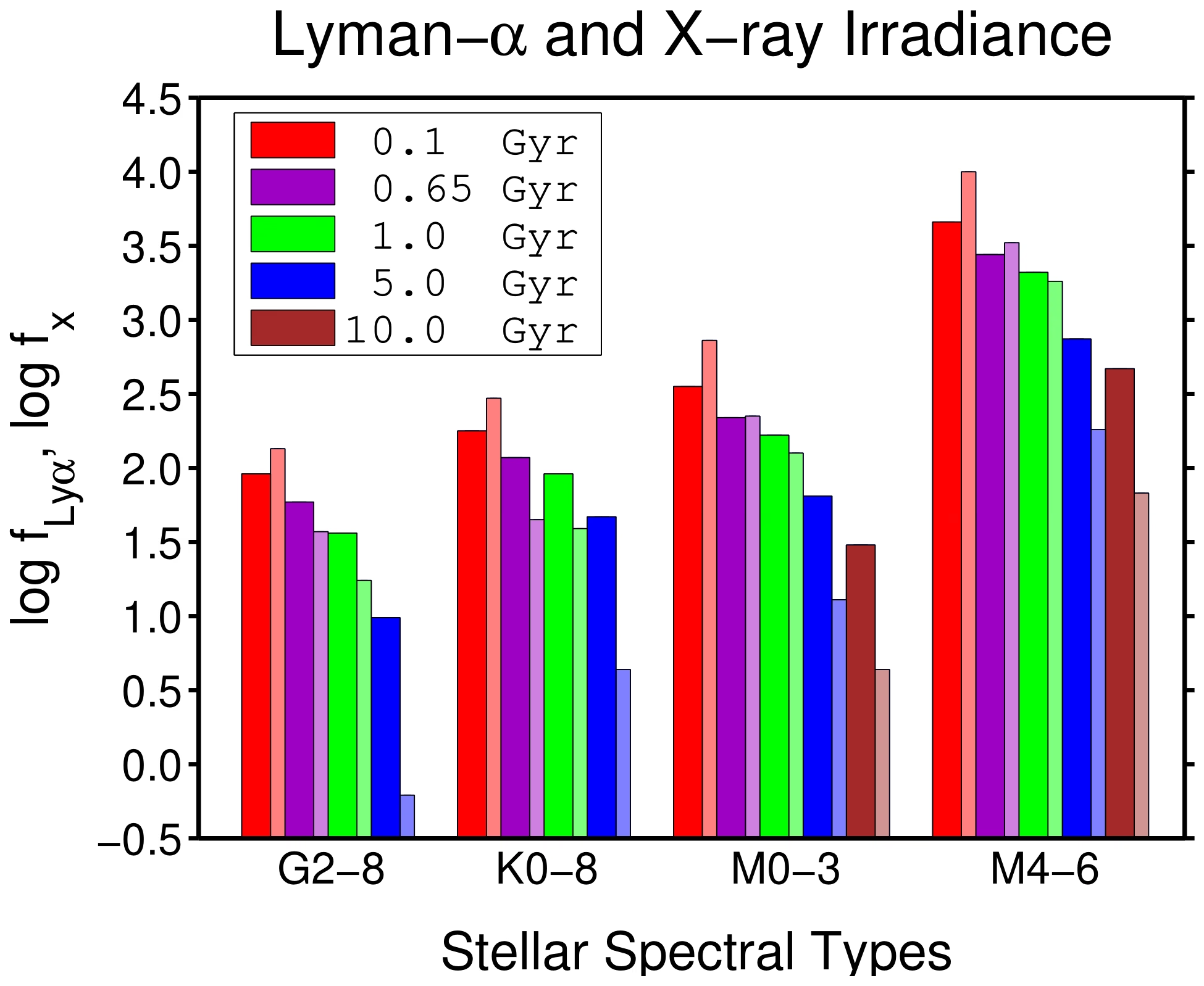
Fig. 14.24 Lyman-\(\alpha\) and X-ray irradiances, in erg s\(^{-1}\) cm\(^{-2}\), received by a planet at the homeothermic distance of its star, the distance at which it absorbs the same flux as Earth does from the Sun. Bars are grouped by spectral type and coloured by stellar age; the wide bar of each pair is Lyman-\(\alpha\) and the narrow, paler bar is X-ray. Note the logarithmic vertical axis. In the plotted bars, the irradiance at fixed age is about 50 to 300 times higher for M4-M6 dwarfs than for G2-G8 dwarfs, and for a given spectral type the X-ray irradiance falls by up to about 200 times between 0.1 and 5 Gyr, while the Lyman-\(\alpha\) decline is much gentler (up to about 10 times). Early K dwarfs are the compromise Cuntz and Guinan [2016] favour: long-lived and common, but without the extreme and long-lasting high-energy irradiation of the M dwarfs. Reproduced from Cuntz and Guinan [2016].

The 1D values listed above for \(d_{\rm in}\) are themselves a simplification. Three-dimensional global climate models that resolve clouds give a different answer for tidally locked planets around M dwarfs. Yang et al. [2013] showed that on a planet that always presents the same face to its star, strong convection at the substellar point lifts thick water clouds that drive the local albedo above \(\sim 0.6\) and act as a stabilising feedback against runaway warming (Fig. 14.25). The result is that the inner edge of the HZ, defined as the largest stellar flux at which surface temperature stays below the runaway threshold, shifts inward by roughly a factor of two relative to the 1D Kopparapu boundary. The 1D HZ therefore under-estimates the inner edge of the M-dwarf HZ, and the corresponding occurrence of habitable planets around M dwarfs is correspondingly larger than the 1D values would suggest.

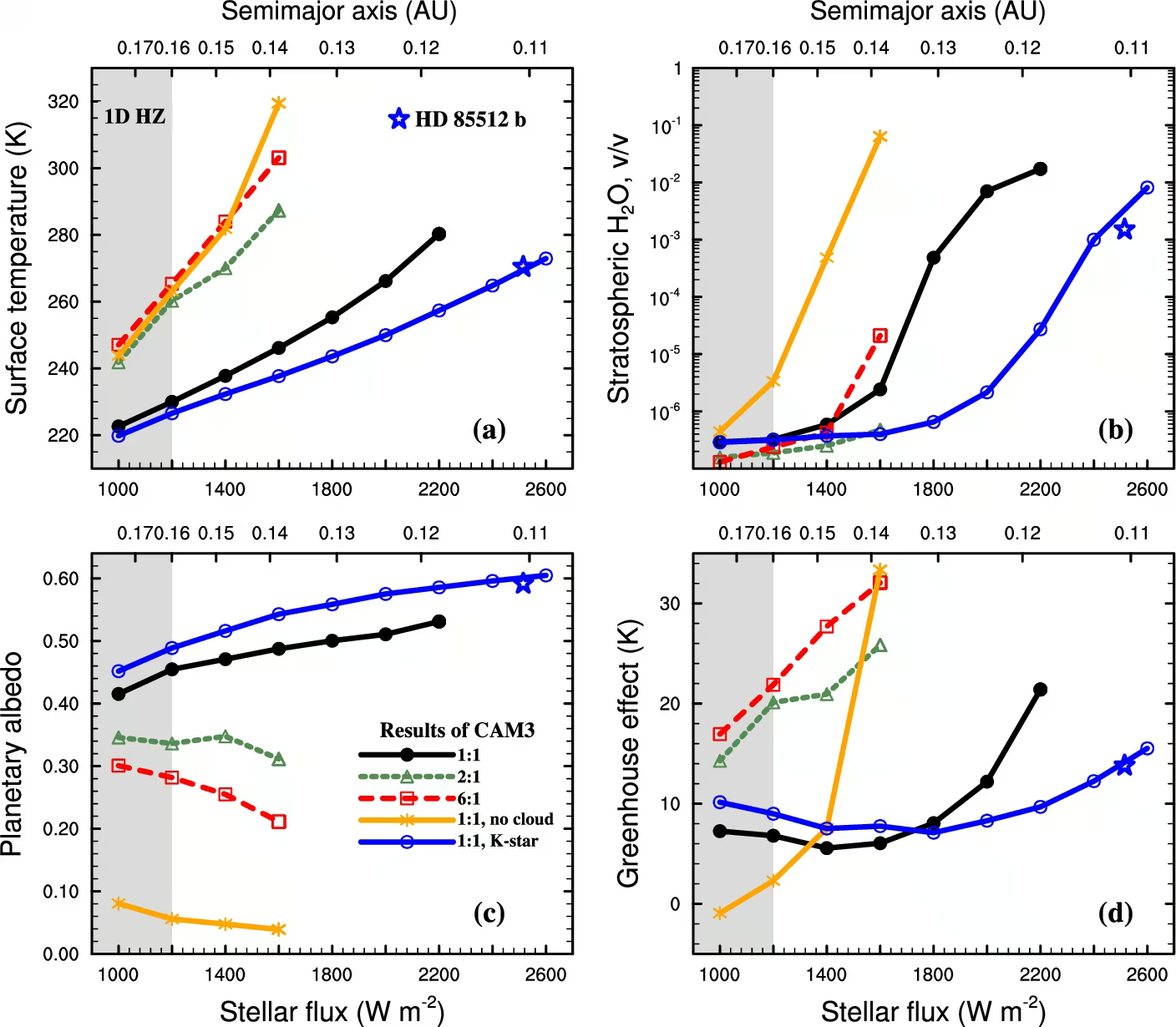
Fig. 14.25 Climates of tidally locked and non-tidally locked rocky planets against incident stellar flux, from the 3D general-circulation model (CAM3) with clouds of Yang et al. [2013] Fig. 2. (a) Global-mean surface temperature, (b) stratospheric water vapour mixing ratio at the substellar point, (c) planetary albedo, and (d) global-mean greenhouse effect, for an M-dwarf host in the spin-orbit states 1:1 (tidally locked, black), 2:1 (green) and 6:1 (red dashed), a 1:1 case with clouds switched off (orange), and a 1:1 case around a K dwarf (blue; the star marks HD 85512 b). The grey band marks the 1D habitable zone. Substellar convective clouds raise the planetary albedo of the tidally locked planet to about 0.5 around the M dwarf (0.6 around the K dwarf) and keep the climate stable up to nearly twice the 1D inner-edge flux; with clouds switched off the albedo drops to 0.04 and the stratosphere becomes moist at much lower flux. Reproduced from Yang et al. [2013].

The combined effect of these climatological corrections is captured in the Shields et al. [2016] summary diagram (Fig. 14.26), which compiles the 1D Kopparapu boundaries together with 3D GCM corrections from a number of independent groups and overlays the known M-dwarf and FGK habitable-zone planets. The figure makes two points at once. First, the 3D inner edge for slowly rotating and tidally locked planets lies at roughly 1.7 to 2.2 times the flux of the 1D inner edge across the whole FGKM range, so it is well inside it. Second, the tidal-locking radius (grey dashed curve) cuts across the M-dwarf HZ, so essentially every M-dwarf HZ planet known today is tidally locked and is therefore in the regime where the cloud corrections matter.

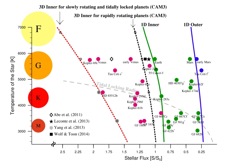
Fig. 14.26 Habitable-zone limits in the plane of stellar effective temperature and stellar flux for FGKM hosts, from the Shields et al. [2016] review of M-dwarf habitability. Note that stellar flux increases to the left. The green and blue solid curves are the Kopparapu et al. [2013] 1D inner (runaway greenhouse) and outer (maximum-\(\mathrm{CO_2}\) greenhouse) edges. The two dotted curves are inner edges computed with the CAM3 general-circulation model: red for slowly rotating and tidally locked planets, black for rapidly rotating planets. The grey dashed curve is the tidal-locking radius. Single-model inner-edge estimates are plotted as the legend symbols, for a dry planet around a G dwarf (Abe et al. 2011), for Earth with the LMD Generic model (Leconte et al. 2013), from Yang et al. [2013], and with a modified radiative-transfer code (Wolf & Toon 2014). Filled circles are solar system planets, including early Venus and early Mars, and known exoplanets; magenta marks those interior to the 1D inner edge and green those within the 1D habitable zone. The red curve lies at about 1.7 to 2.2 times the flux of the green one, so clouds move the inner edge substantially closer to the star, and that is the regime almost every M-dwarf planet in the figure occupies. Reproduced from Shields et al. [2016], after Yang et al. (2014).

The tidal-locking radius itself is not a free parameter: it follows from how fast tides can despin a rotating planet. For a rocky planet of mass \(M_p\), radius \(R_p\), moment of inertia \(I_p \approx \alpha_p M_p R_p^2\) (with the dimensionless moment-of-inertia factor \(\alpha_p \approx 0.33\) for an Earth-like differentiated body), tidal Love number \(k_{2,p}\), and quality factor \(Q_p\), orbiting a star of mass \(M_\star\) at semi-major axis \(a\), the timescale to despin from an initial spin rate \(\omega_0\) to synchronous rotation is, to order of magnitude,

\[ \tau_{\rm lock} \;\sim\; \frac{\omega_0 \, a^6 \, I_p \, Q_p}{3 \, G \, M_\star^2 \, k_{2,p} \, R_p^5} \,. \]

The strong \(a^6\) dependence (an inverse-cube tidal force squared) means the answer changes by many orders of magnitude across the HZ. Plugging in Earth-like parameters (\(\alpha_p \approx 0.33\), \(k_{2,p} \approx 0.3\), \(Q_p \approx 100\), \(\omega_0 \sim 2\pi/(\text{day})\)) for an Earth analogue at \(a = 1\) AU around the Sun gives \(\tau_{\rm lock} \sim 10^{11}\) yr, several times the age of the universe, so an Earth analogue at 1 AU around a Sun-like star is not tidally locked. For a TRAPPIST-1 b analogue, however, \(a \approx 0.011\) AU and \(M_\star \approx 0.09\,\Msun\) shrink the numerator and the denominator together; the strong \(a^6\) scaling dominates, so the net effect is that \(\tau_{\rm lock}\) drops by nearly ten orders of magnitude to decades (the precise value scales with the highly uncertain \(Q_p\), and even \(Q_p \sim 10^3\) gives only centuries), which is in any case far shorter than the \(\sim 8\) Gyr age of the TRAPPIST-1 system. Every TRAPPIST-1 inner planet has therefore had ample time to reach a tidally locked or near-locked spin state, and the same conclusion holds for essentially every M-dwarf HZ planet known today. The 3D climate corrections shown above are not an academic complication: they apply to the regime in which essentially all M-dwarf HZ planets sit.

Key insight. The HZ as derived above is a useful 1D radiative limit. It is well-defined as a thermodynamic boundary on the location of liquid surface water, but it is not a sufficient condition for habitability. Real habitability also depends on planetary boundary conditions (volatile inventory, tectonic regime, escape history, magnetic shielding, evolutionary trajectory) that the 1D HZ ignores. Part 2’s coupling loop is the qualitative version of what a full 3D climate-evolution model computes quantitatively for an individual planet.

14.4. Part 3: Astrobiology and the search for life

14.4.1. What is life?

Astrobiology operates without an agreed-upon definition of life. The working definition, going back to Lederberg [1965], is that life is a self-replicating, metabolising, evolving chemical system. This operational definition lets us decide what to look for.

The search for life elsewhere is dominated by carbon-based, water-as-solvent biology because we know its spectroscopic and geochemical fingerprints. Alternative biochemistries (silicon-based, ammonia-solvent, methane-solvent) are not excluded in principle, but they are not our default working hypothesis.

Fig. 14.27 summarises this working definition.

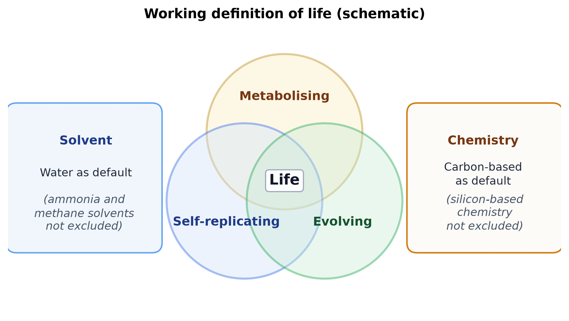
Fig. 14.27 The working definition of life used in this course: a chemical system that is self-replicating, metabolising and evolving. Water is the default solvent and carbon the default chemistry, but silicon-based chemistry and ammonia or methane solvents are not excluded in principle. Course-original figure.

14.4.2. Extremophiles and the redefinition of “habitable”

Historically, the operational definition of “habitable” assumed conditions under which temperate Earth surface organisms thrive. The discovery of extremophiles, organisms thriving far outside that range, has substantially relaxed this definition.

Earth life occupies environments from hydrothermal vents over 120 \(^\circ\)C to Arctic permafrost brines, where bacteria still grow at \(-15\) \(^\circ\)C and remain metabolically active at \(-25\) \(^\circ\)C, as well as saturated brine and hyperacidic drainage. The implication for astrobiology is that the classical HZ, defined for surface liquid water on a temperate Earth-like planet, may be too restrictive. Subsurface oceans on icy moons and high-pressure environments cannot be excluded on energetic grounds.

Icy moons (Europa, Enceladus, Titan) became primary astrobiology targets, formalised in NASA’s Roadmap to Ocean Worlds [Hendrix et al., 2019]. None are in the classical HZ, yet all have liquid water and a chemical free-energy gradient: Europa and Enceladus with the water in contact with rock, Titan with its ocean on a layer of high-pressure ice (Lecture 8, Lecture 11).

Fig. 14.28 compares the temperature range of Earth life with the temperate surface conditions that the classical definition assumed.

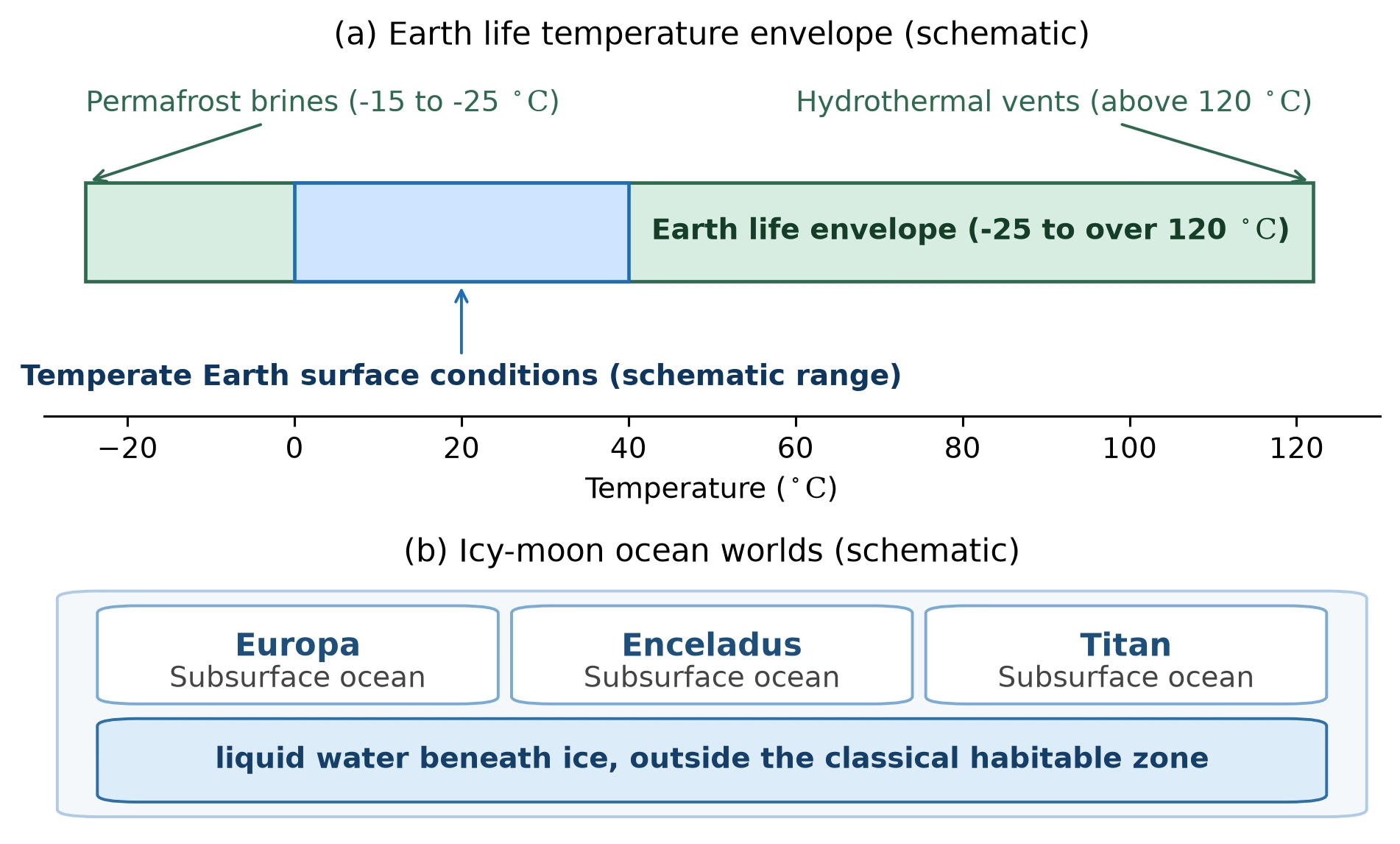
Fig. 14.28 Extremophiles widen the definition of habitable. (a) The temperature range of Earth life, from permafrost brines at \(-15\) to \(-25\) \(^\circ\)C to hydrothermal vents above \(120\) \(^\circ\)C, compared with the temperate surface conditions that the classical definition of habitability assumed (inner bar, schematic range). (b) The icy moons Europa, Enceladus and Titan hold subsurface oceans beneath ice and lie outside the classical habitable zone; at Europa and Enceladus the water touches rock, at Titan it rests on high-pressure ice. Course-original figure.

14.4.3. Origin of life on Earth

The origin of life on Earth remains an unsolved scientific problem (the Precambrian record is in Lecture 9) with several competing hypotheses:

• RNA world: the hypothesis that self-replicating RNA preceded protein-based metabolism. This model is supported by catalytic ribozymes in modern organisms and the ribosome, but prebiotic nucleotides do not easily polymerise without templating and are unstable on long timescales.

• Metabolism-first: the hypothesis that chemical autocatalytic cycles preceded genetic information storage. Submarine alkaline hydrothermal vents produce \(\mathrm{H_2}\), methane, and redox disequilibrium gradients between fluid and seawater that resemble primitive metabolism [Russell et al., 2014].

• Surface “warm little ponds”: the hypothesis that wet-dry cycling in shallow surface pools concentrates and polymerises prebiotic nucleotides [Sasselov et al., 2020].

• Panspermia: the hypothesis that life arrived on meteorites or comets, which relocates the origin question to another planetary body rather than solving it.

The earliest direct evidence of life on Earth dates to about 3.5 Ga from microbial mat structures in Australia and South Africa. Possible isotopic and morphological biosignatures have been claimed at \(\sim 3.8\) Ga in Isua banded iron formations [Mojzsis et al., 1996] and, more controversially, up to \(\sim 4.3\) Ga in the Nuvvuagittuq Supracrustal Belt (minimum age \(\sim 3.77\) Ga) [Dodd et al., 2017]. If validated, life arose within a few hundred Myr of the cooling of Earth’s surface, early in Earth’s geologic history (Fig. 14.29).

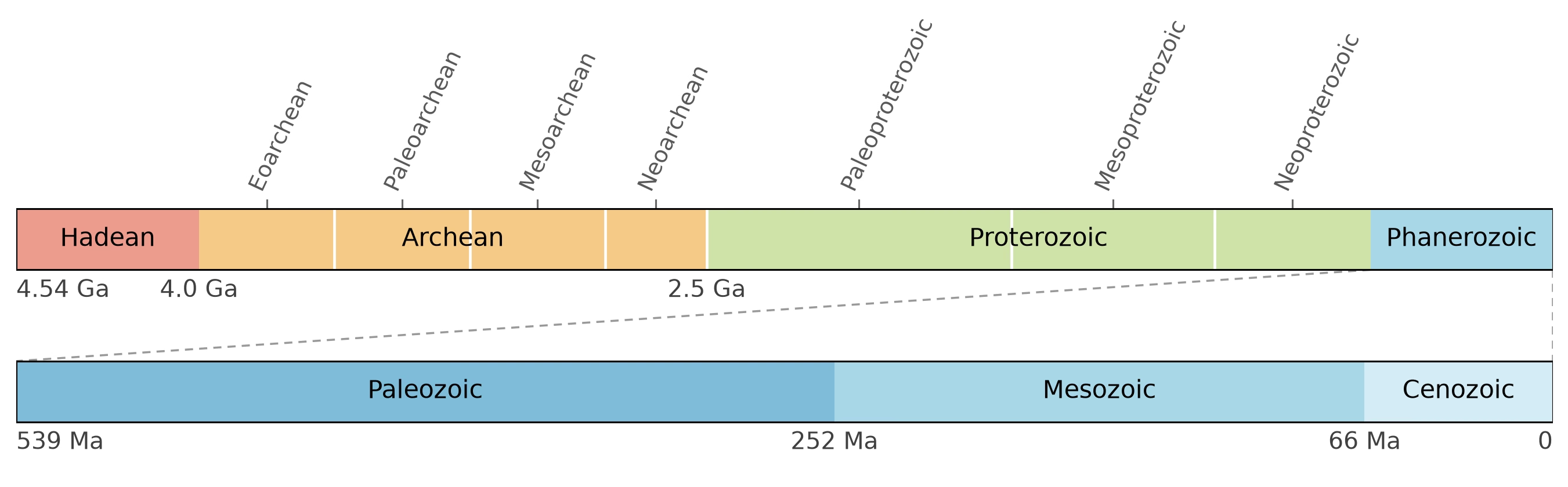
Fig. 14.29 The geologic eons and eras of Earth. Top bar: the four eons spanning the full \(4.54\) Gyr of Earth history, with the eras of the Archean and Proterozoic marked above; note that the Hadean, Archean, and Proterozoic together (the informal “Precambrian”) occupy almost \(90\%\) of the timeline. Bottom bar: the Phanerozoic eon stretched to the full figure width, divided into the Paleozoic, Mesozoic, and Cenozoic eras at the end-Permian (\(252\) Ma) and end-Cretaceous (\(66\) Ma) mass extinctions. Boundary ages follow the Geologic Time Scale 2020 [Gradstein et al., 2020]. Course-original figure.

The unknown frequency of abiogenesis represents the largest uncertainty in quantitative habitability estimates, leaving \(f_l\) in the Drake equation unconstrained. A second independent origin of life on Mars or an icy moon would provide the first empirical constraint on \(f_l\).

14.4.4. Biosignatures: what would we look for?

A biosignature is an observable feature whose presence is more easily explained by biology than by abiotic processes alone. Schwieterman et al. [2018] divide remotely detectable biosignatures into atmospheric gases, surface reflectance features, and temporal variability (Fig. 14.32). Catling et al. [2018] lay out an assessment framework for candidate biosignatures and evaluate them within a Bayesian framework that updates the probability of life given planetary and stellar context (Fig. 14.30).

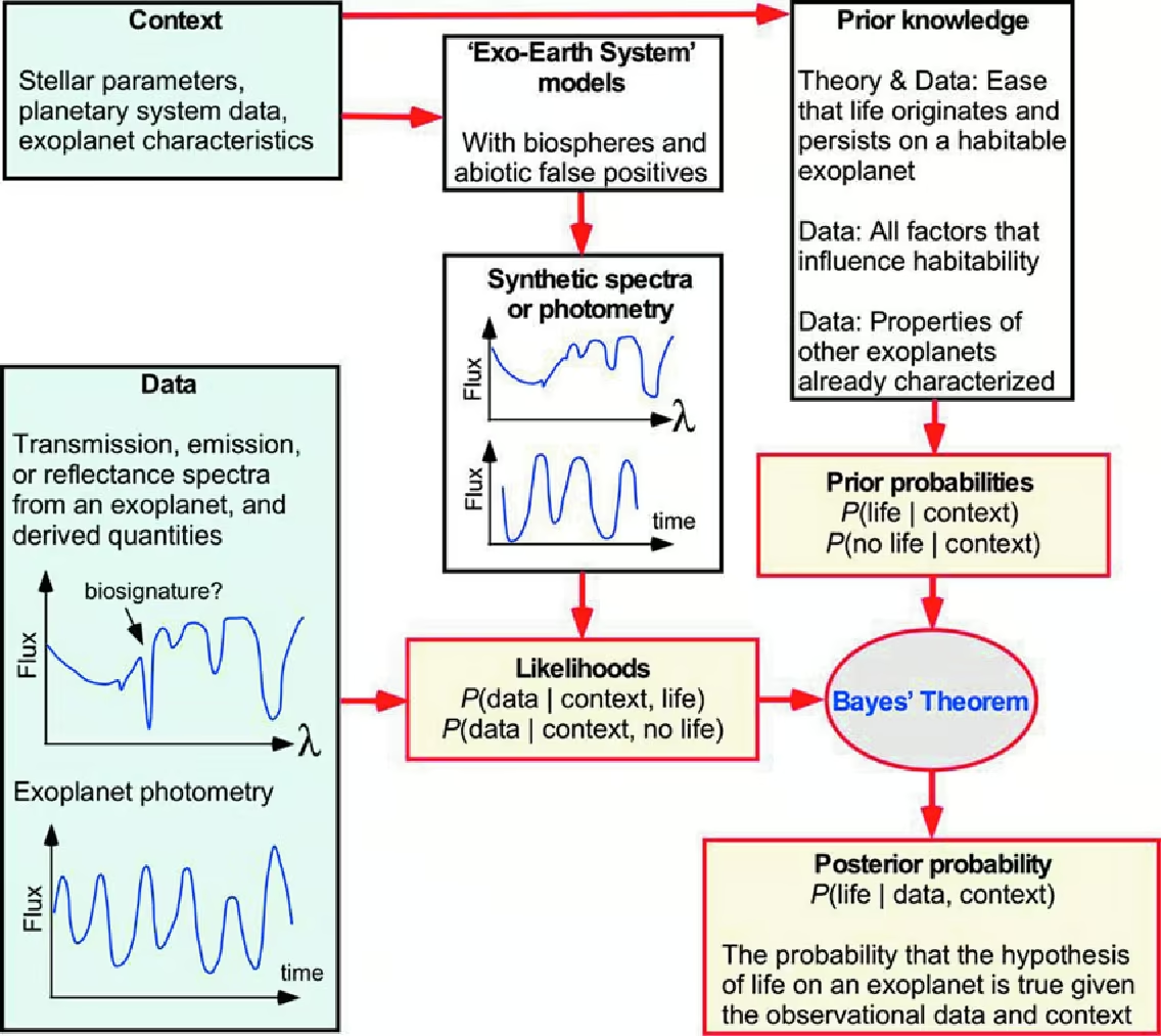
Fig. 14.30 A Bayesian framework combines exoplanet observations with theoretical and population priors to compute the posterior probability of life. Detection is a quantitative inference from a chain of measurements rather than a single observation; reproduced from Catling et al. [2018].

On Earth, single gas biosignatures include \(\mathrm{O_2}\) (\(\sim 21\%\)), photochemical \(\mathrm{O_3}\), biogenic \(\mathrm{CH_4}\), and \(\mathrm{N_2O}\). The most diagnostic signatures are combinations in chemical disequilibrium, where coexisting gases react rapidly and require continuous resupply. Krissansen-Totton et al. [2016] calculated an available Gibbs energy of about 2326 J/mol for the atmosphere-ocean system of modern Earth, mainly from \(\mathrm{N_2}\) and \(\mathrm{O_2}\) coexisting with liquid water, compared to about 136 J/mol for the atmosphere of Mars, the largest of any other solar system atmosphere. Earth’s atmosphere alone holds only about 1.5 J/mol, less than Mars: the ocean makes the difference. On the Archean Earth (roughly 4.0 to 2.5 billion years ago), coexisting \(\mathrm{CH_4}\), \(\mathrm{CO_2}\), \(\mathrm{N_2}\), and liquid \(\mathrm{H_2O}\) formed a disequilibrium biosignature that cannot persist abiotically (Fig. 14.31).

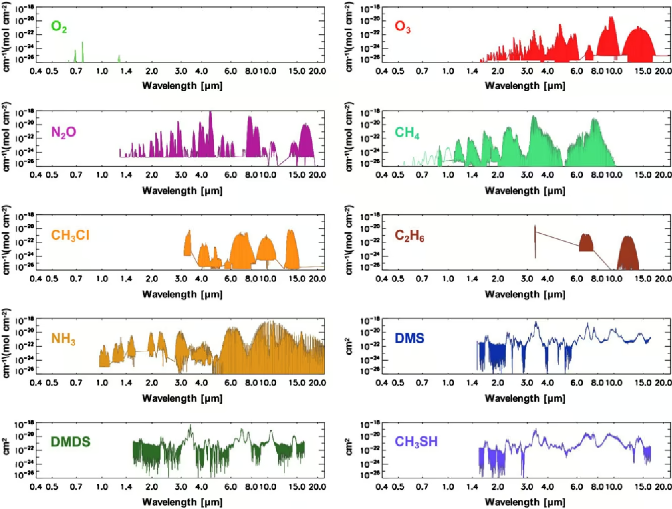
Fig. 14.31 Wavelength-resolved infrared absorption spectra from \(0.4\) to \(20\,\mu\mathrm{m}\) for ten potential biosignature gases. Diagnostic bands include \(\mathrm{O_3}\) near \(9.6\,\mu\mathrm{m}\), \(\mathrm{CH_4}\) at \(3.3\) and \(7.7\,\mu\mathrm{m}\), \(\mathrm{N_2O}\), and DMS/DMDS in the \(6\) to \(15\,\mu\mathrm{m}\) window; reproduced from Schwieterman et al. [2018].

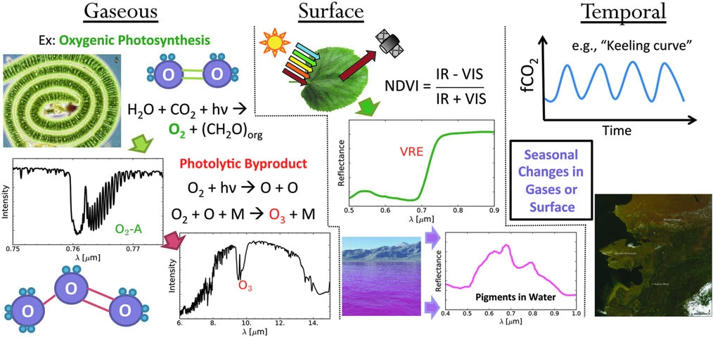
Fig. 14.32 The three classes of remotely detectable biosignatures comprise gaseous by-products, surface pigment features, and temporal variations. A convincing biosignature claim ideally combines evidence across multiple classes to exclude abiotic false positives; reproduced from Schwieterman et al. [2018].

Surface biosignatures include the vegetation red edge, a sharp reflectance jump at \(\sim 700\) nm from chlorophyll, while temporal biosignatures comprise seasonal cycles in atmospheric gases and surface reflectance.

14.4.5. False positives and the inverse problem

Most candidate biosignature gases have a known abiotic production pathway under plausible planetary conditions [Meadows et al., 2018]:

• Abiotic \(\mathrm{O_2}\) from photolysis (the breakdown of a molecule by absorbed stellar light) of \(\mathrm{H_2O}\) followed by hydrogen escape: around any star type when the atmosphere holds little \(\mathrm{N_2}\) or other non-condensing gas, so that the cold trap fails [Wordsworth and Pierrehumbert, 2014], and during the long runaway phase of planets around young M dwarfs [Luger and Barnes, 2015]; \(\mathrm{CO_2}\) photolysis is a further abiotic source.

• Abiotic \(\mathrm{CH_4}\) from serpentinisation (the reaction of olivine with water to form serpentine minerals and release hydrogen), or volcanic outgassing at low oxygen fugacity.

• Abiotic \(\mathrm{N_2O}\) from lightning chemistry and photochemical pathways.

• Dimethyl sulfide (\(\mathrm{(CH_3)_2S}\), DMS) is the notable exception: it lacks known abiotic sources on Earth, but one could exist elsewhere.

Biosignature detection is therefore an inverse problem: a single detection cannot prove life. Reliable life detection requires context, gas combinations, and multi-wavelength observations that constrain planetary state, escape history, and atmospheric composition together (Fig. 14.33).

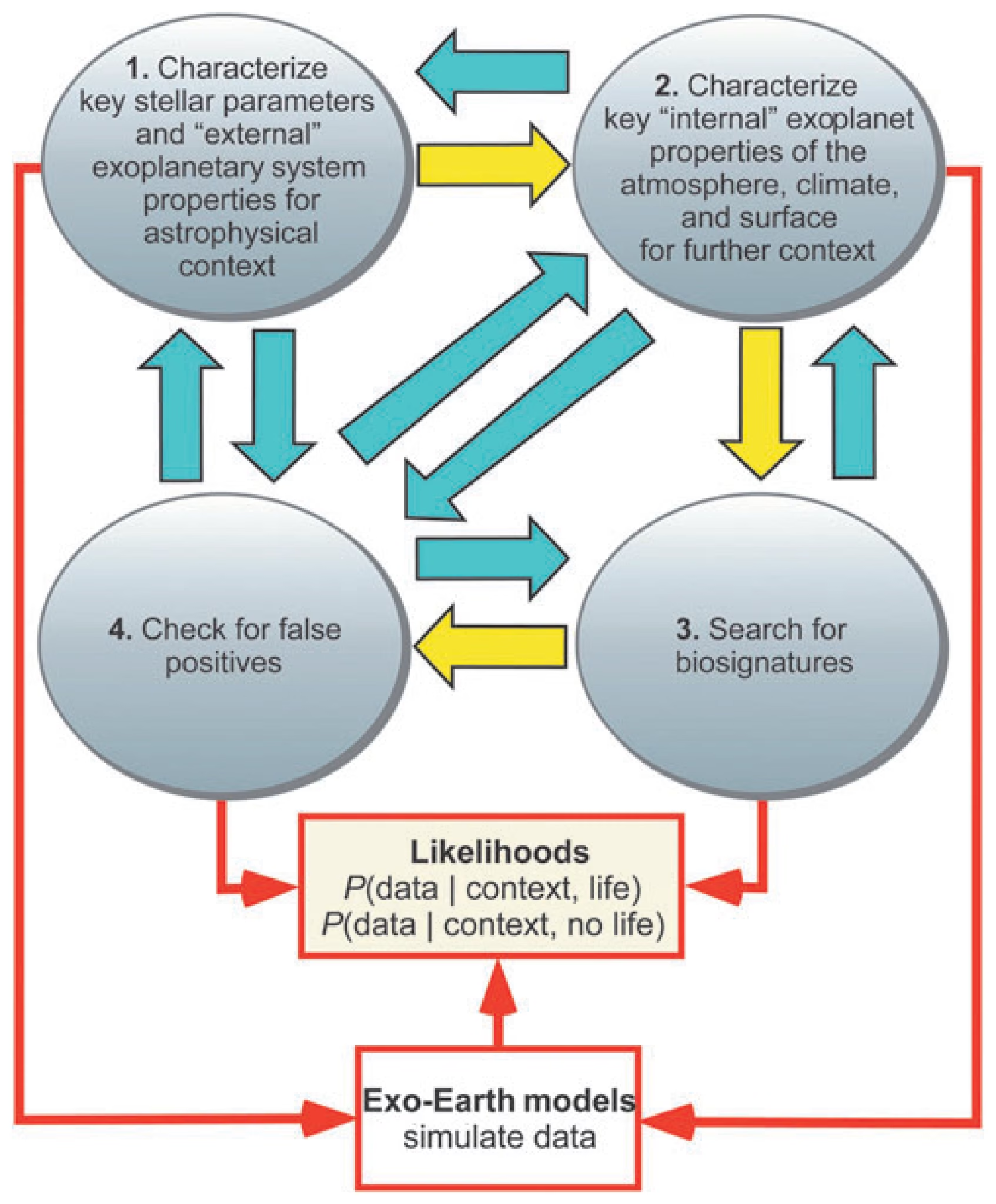
Fig. 14.33 The four-component framework for assessing exoplanet biosignatures from Catling et al. [2018]. Component 1 (top left) characterises the host star and the external properties of the planetary system; component 2 (top right) characterises the internal properties of the planet: atmosphere, climate, and surface. Component 3 (bottom right) is the search for biosignatures, and component 4 (bottom left) the check for false positives. Yellow arrows mark an idealised observing sequence; blue arrows mark the iterations that raise confidence in a biosignature or expose a false positive. Combined with exo-Earth models that simulate the data, the four components constrain the likelihoods of the data with and without life (red boxes). Reproduced from Catling et al. [2018].

14.4.6. Solar system targets for life detection

The solar system contains five plausible targets for life detection.

Mars (Lecture 10) is the most direct path to laboratory-based life detection on another world. Curiosity and Perseverance established that Mars had liquid water, neutral pH, and complex organic molecules at \(\sim 3.5\) to \(4\) Ga. Present-day habitability is more uncertain: the methane variability detected by Curiosity is intriguing but cannot be interpreted as biological without independent corroboration. Laboratory analysis of returned samples in full spatial and chemical context remains the most direct test [Meyer et al., 2022], but the samples cached by Perseverance stay on Mars for now: the NASA and ESA Mars Sample Return campaign received no funding in the US budget for 2026.

Europa (Lecture 11) has a global subsurface saltwater ocean confirmed by Galileo induced magnetic field measurements and surface brine chemistry; Europa Clipper (arriving 2030) and JUICE (Ganymede orbit 2034) will measure the ice-shell thickness and ocean properties.

Enceladus (Lecture 11) ejects samples of its subsurface ocean directly into space through its south-polar plume. Cassini detected \(\mathrm{H_2}\) from active serpentinisation at the rocky core, macromolecular organics, and sodium phosphates indicating phosphorus-rich ocean chemistry [Postberg et al., 2018, Postberg et al., 2023, Waite et al., 2017].

Titan (Lecture 11) is the only body other than Earth with stable surface liquids today, featuring methane and ethane lakes and active prebiotic photochemistry. NASA’s Dragonfly rotorcraft (launch 2028, arrival 2034) will sample the organic-rich surface (Lecture 11).

Venus cloud layer. Greaves et al. [2021] claimed phosphine (\(\mathrm{PH_3}\)) in the temperate cloud deck at altitudes of \(50\) to \(60\) km as a possible biosignature lacking known abiotic sources. Reanalyses of JCMT and ALMA data showed the spectral feature was at the instrumental sensitivity limit and consistent with mesospheric \(\mathrm{SO_2}\) [Lincowski et al., 2021] (Fig. 14.34). Independent observations failed to confirm the detection, setting lower upper limits.

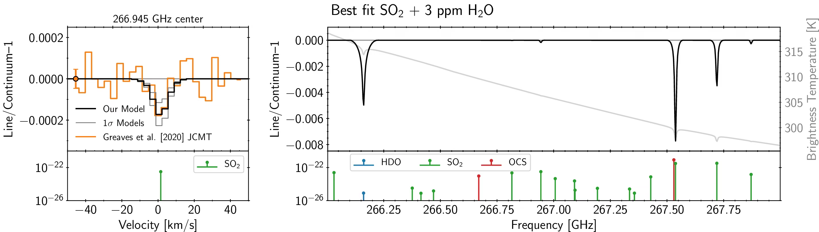
Fig. 14.34 Spectral simulations of the 266.94 GHz feature claimed as \(\mathrm{PH_3}\) in the Venus clouds, showing that the same data are also consistent with mesospheric \(\mathrm{SO_2}\) at the few-hundred-ppb level (rising from \(\sim 30\) ppb at 78 km to \(\sim 400\) ppb at 100 km altitude). The original Greaves et al. [2021] detection sits at the edge of the instrumental noise floor and the alternative \(\mathrm{SO_2}\) interpretation cannot be excluded. Reproduced from Lincowski et al. [2021].

The Venus phosphine episode parallels the K2-18 b DMS controversy on the exoplanet side. In both cases, data at instrumental sensitivity limits allow plausible abiotic explanations that have not been ruled out. Extraordinary claims about biosignatures require extraordinary verification through independent datasets.

The upcoming Venus missions DAVINCI (in situ), EnVision, and VERITAS (from orbit) will provide higher-precision data (Lecture 9).

Pedagogical point. The Venus phosphine and K2-18 b DMS cases show that claims about life-relevant chemistry must clear a high bar through better data rather than rhetoric. Both controversies drive the design of next-generation instruments and missions.

14.4.7. Exoplanet life detection: the strategy

Exoplanet life detection relies entirely on spatially unresolved transmission, emission, or reflectance spectra (Lecture 13) (Fig. 14.35).

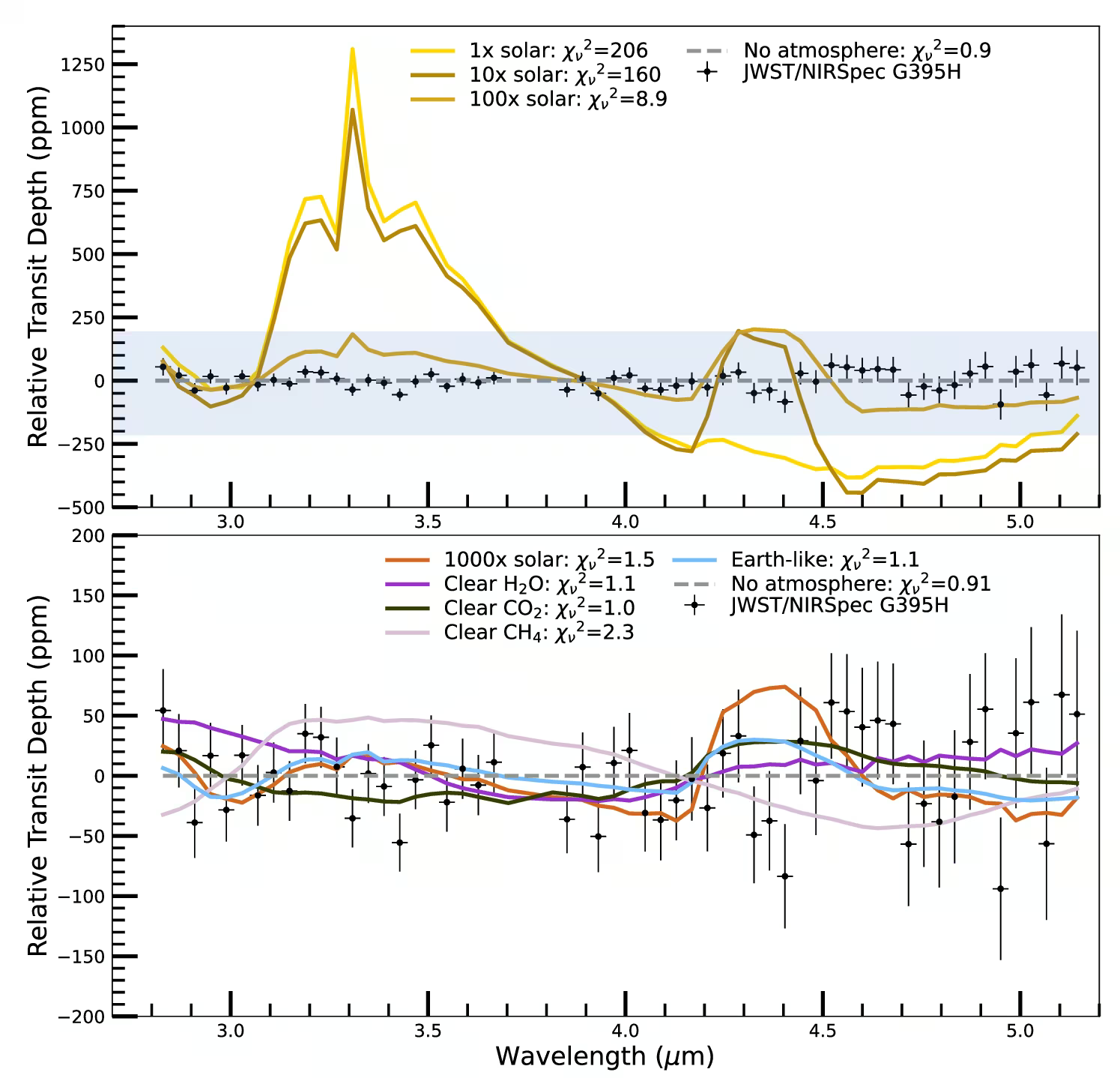
Fig. 14.35 JWST/NIRSpec G395H transmission spectrum of the Earth-sized rocky exoplanet LHS 475 b (black points), compared with model atmospheres of various compositions. The data rule out clear hydrogen-dominated atmospheres at \(1\times\) to \(100\times\) solar metallicity at high significance (top panel). High mean molecular weight atmospheres (pure \(\mathrm{H_2O}\), \(\mathrm{CO_2}\)-dominated, Earth-like) and a featureless airless-body spectrum remain consistent with the data, while a clear \(\mathrm{CH_4}\)-dominated atmosphere is weakly disfavoured (bottom panel). This is representative of what current JWST observations can and cannot say about the atmospheres of rocky exoplanets around nearby M dwarfs. Reproduced from Lustig-Yaeger et al. [2023].

For TRAPPIST-1 b, the degeneracy of a featureless transmission spectrum was broken by MIRI \(15\,\mu\mathrm{m}\) secondary eclipse observations: a dayside brightness temperature \(T_d \approx 503\) K matches the \(508\) K expected for bare rock without heat redistribution (Fig. 14.36; Lecture 13).

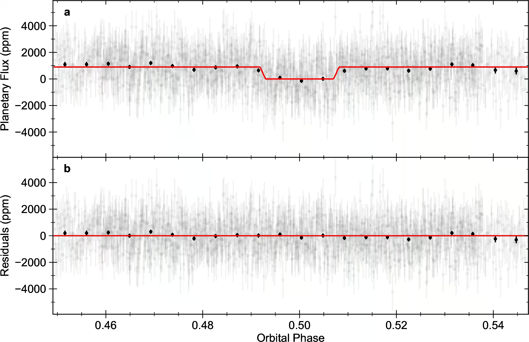
Fig. 14.36 JWST MIRI secondary eclipse light curve of TRAPPIST-1 b at 15 \(\mu\)m. The observed eclipse depth corresponds to a measured dayside brightness temperature of \(T_d \approx 503\) K, consistent with the 508 K bare-rock zero-redistribution prediction and indicating that the planet has no thick atmosphere to redistribute heat. Reproduced from Greene et al. [2023].

The K2-18 b transmission spectrum in Fig. 14.37 shows what such a molecular detection looks like.

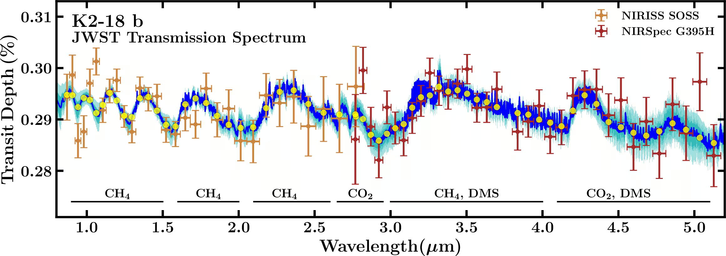
Fig. 14.37 JWST transmission spectrum of K2-18 b from Madhusudhan et al. [2023]. The combined NIRSpec and NIRISS data show clear \(\mathrm{CH_4}\) and \(\mathrm{CO_2}\) absorption features and the tentative DMS feature near 3.4 \(\mu\)m. The spectrum is consistent with a sub-Neptune atmosphere overlying either a “hycean” (hydrogen atmosphere over a global liquid-water ocean) layer or a deeper mini-Neptune envelope. Reproduced from Madhusudhan et al. [2023].

As shown for K2-18 b in Lecture 13, a single-snapshot atmospheric detection is insufficient to establish the presence of biology (Fig. 14.38).

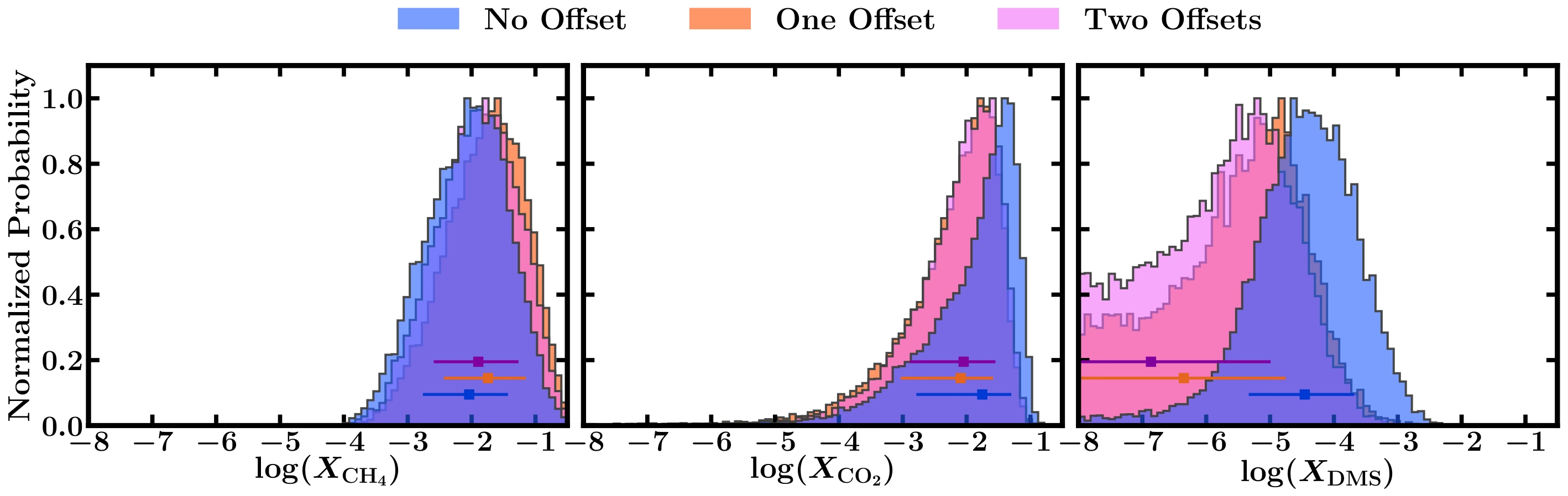
Fig. 14.38 Posterior probability distributions for the mixing ratios of \(\mathrm{CH_4}\), \(\mathrm{CO_2}\), and DMS in the atmosphere of K2-18 b, for three retrievals that differ only in how many instrument offsets are allowed to float: none (blue), one (orange), and two (pink). The horizontal bars give each distribution’s median and \(1\sigma\) interval. \(\mathrm{CH_4}\) and \(\mathrm{CO_2}\) are recovered at about \(5\sigma\) and \(3\sigma\) and their posteriors shift only slightly between the three cases. The DMS posterior behaves in the opposite way: \(2.4\sigma\) with no offset, about \(1\sigma\) with one, and no longer significant with two. That sensitivity to a nuisance parameter is exactly the inverse-problem issue that makes single-snapshot biosignature claims hard to validate. Reproduced from Madhusudhan et al. [2023].

A convincing biosignature detection requires chemical disequilibrium, temporal variability, environmental context excluding abiotic pathways, and independent confirmation. The Habitable Worlds Observatory (HWO; National Academies of Sciences, Engineering, and Medicine [2021]) will use a \(\sim 6\) m space-based coronagraph (an instrument masking starlight to image faint planets) to characterise Earth-like planets around \(\sim 25\) Sun-like stars in the 2040s. The proposed mid-infrared interferometer LIFE (Large Interferometer For Exoplanets) would target the thermal-infrared bands of biosignature gases such as \(\mathrm{O_3}\), \(\mathrm{CH_4}\) and \(\mathrm{N_2O}\) [Quanz et al., 2022].

Dedicated exoplanet life-detection flagships are expected in the 2040s following 2030s statistical surveys. Future observatories will constrain \(f_l\), transforming the search for life into an empirical science.

14.5. Course wrap-up

14.5.1. The five biggest things we have learned

1. Planet formation is a physical process governed by accretion, gravity, and disk dynamics, producing a predictable diversity of outcomes.

2. Planetary interiors are heat engines whose evolution drives surface tectonics, volcanic outgassing, magnetic dynamos, and long-term habitability on Gyr timescales.

3. Atmospheres are dynamic systems that form, evolve, escape, and react with interiors and surfaces, so no default atmosphere exists.

4. Habitability is a coupled systems property linking stellar, orbital, planetary, and biospheric factors across star, atmosphere, surface, and interior.

5. The solar system is a detailed reference case, while the exoplanet population provides the statistical context for what is typical.

Fig. 14.39 gives one icon per lesson.

Fig. 14.39 The five biggest lessons of the course as icons. (a) Planet formation: accretion from a disk. (b) Planetary interiors: heat engines (core, mantle, heat flux) whose evolution drives tectonics, outgassing and dynamos. (c) Atmospheres: dynamic systems that form, evolve, escape and react with interiors and surfaces. (d) Habitability: a coupled property of star, atmosphere, surface and interior. (e) The solar system: a detailed reference case, with the exoplanet population as the statistical context. Course-original figure.

14.5.2. The five biggest open questions

1. Whether the origin of life is a rare accident or a generic chemical inevitability remains the largest uncertainty in quantitative habitability estimates.

2. The radius valley between super-Earths and sub-Neptunes tests whether photoevaporation, core-powered mass loss, or distinct formation channels govern atmospheric loss.

3. When Jupiter formed determines whether it was the architect of the inner solar system, shaping the NC-CC dichotomy and Earth-like system rarity.

4. Returned samples from Mars provide the most direct test of whether Mars was ever inhabited, recalibrating our prior on \(f_l\).

5. Determining whether the solar system is rare or typical using PLATO, Gaia DR4/DR5, and long-baseline RV will yield a probabilistic answer.

Fig. 14.40 pairs each question with what is at stake or with the test that will decide it.

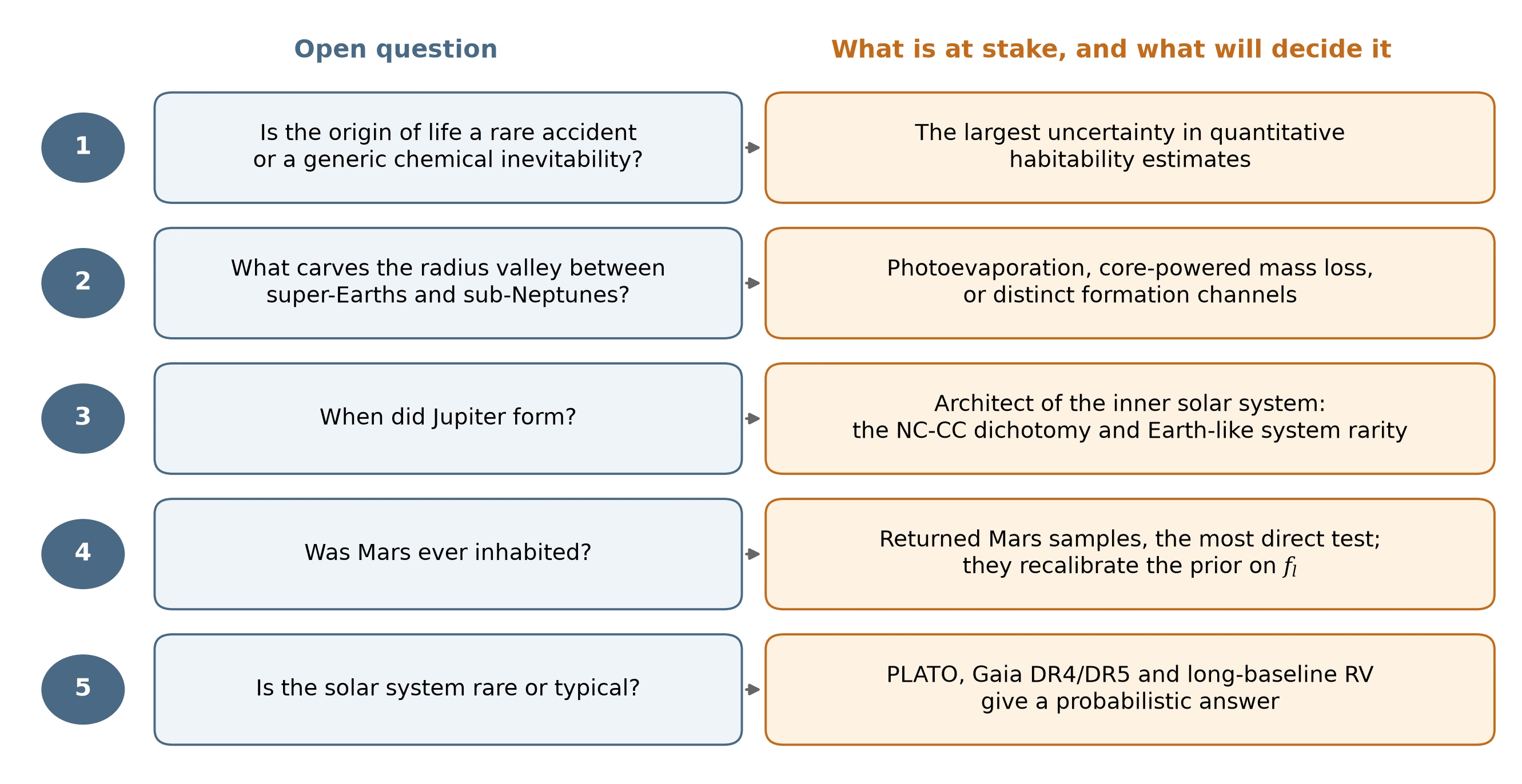
Fig. 14.40 The five biggest open questions of the course, each paired with what is at stake or with the test that will decide it. (1) Whether the origin of life is a rare accident or a generic chemical inevitability, the largest uncertainty in quantitative habitability estimates. (2) Whether photoevaporation, core-powered mass loss or distinct formation channels carve the radius valley. (3) When Jupiter formed, which decides whether it shaped the NC-CC dichotomy and the rarity of Earth-like systems. (4) Whether Mars was ever inhabited, with returned samples as the most direct test. (5) Whether the solar system is rare or typical, which PLATO, Gaia DR4/DR5 and long-baseline radial-velocity surveys will answer probabilistically. Course-original figure.

14.5.3. The next decade

The most decisive advance in exoplanet characterisation over the coming decade will come from ground-based 30-metre-class observatories entering operation. With its 39 m segmented primary mirror, ESO’s Extremely Large Telescope (ELT; Fig. 14.41) will be the largest optical and near-infrared telescope ever constructed. Equipped with extreme adaptive optics and high-resolution spectrographs, the ELT will achieve the angular resolution and high contrast required to isolate reflected starlight and thermal emission from planets at small orbital separations. This will enable direct imaging and spectroscopic characterisation of temperate Earth-sized rocky planets in the habitable zones of nearby M dwarfs, testing for atmospheric water vapour, carbon dioxide, and candidate biosignatures.

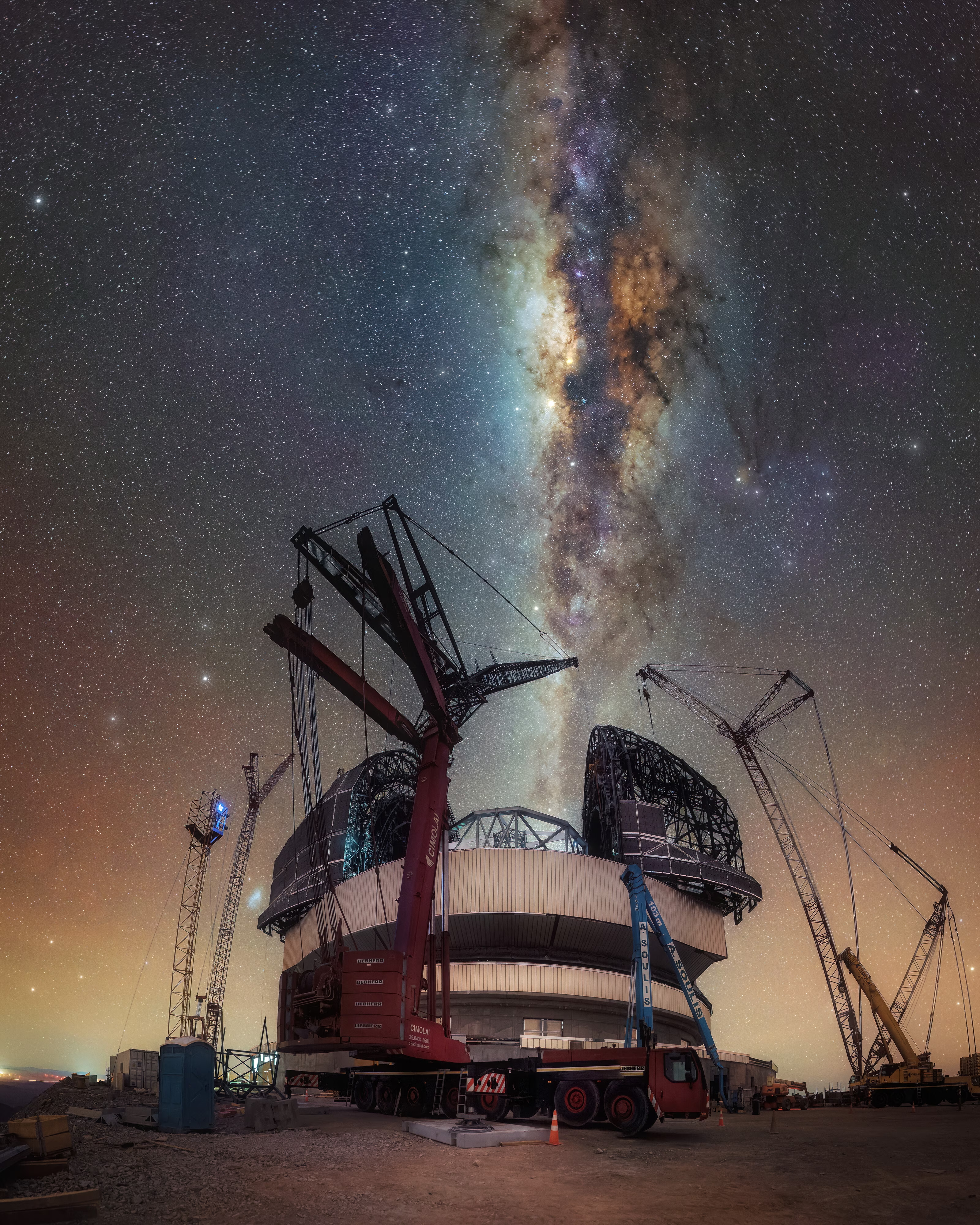
Fig. 14.41 The Milky Way arcs over ESO’s Extremely Large Telescope under construction on Cerro Armazones in the Chilean Atacama Desert, with the partially clad dome in the lower centre (August 2025). With its 39 m segmented primary mirror, the ELT will be the largest optical/near-infrared telescope ever built when it sees first light in 2029 and will, together with GMT and TMT, enable the first direct-imaging searches for atmospheric biosignatures on rocky planets around nearby M dwarfs. Image credit: C. Letelier/ESO [ESO, 2025].

14.5.4. Final framing

Planetary science has become the science of comparative climate, interior, and life-hosting trajectories. The solar system is the reference system (Fig. 14.42), but no longer the benchmark. The exoplanet population provides the statistical context that the solar system on its own cannot. The questions covered across this course are open questions on a moving frontier.

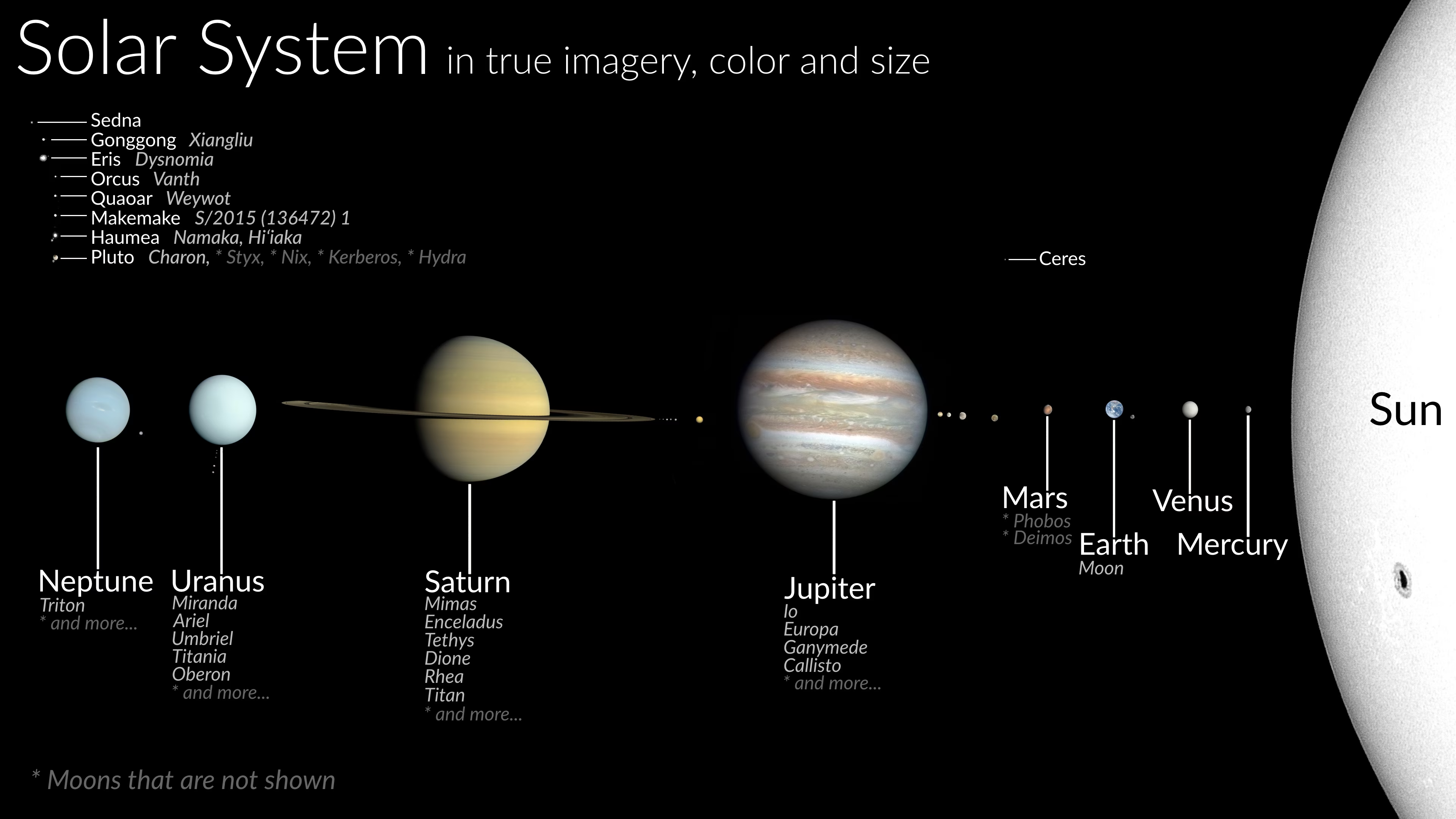
Fig. 14.42 Composite at true relative size of the principal bodies of the solar system, grouped by region. Inner solar system: Mercury, Venus, Earth (with the Moon), and Mars (Phobos and Deimos are listed but not shown). Asteroid belt: represented by the dwarf planet Ceres. Outer solar system: Jupiter, Saturn, Uranus, and Neptune, each shown with their largest moons (Io, Europa, Ganymede, Callisto for Jupiter; Mimas, Enceladus, Tethys, Dione, Rhea, Titan for Saturn; Miranda, Ariel, Umbriel, Titania, Oberon for Uranus; Triton for Neptune). Kuiper Belt, scattered disk, and detached objects: Pluto (with Charon; Styx, Nix, Kerberos, and Hydra are listed but not shown), Haumea (with Namaka and Hi’iaka), Makemake (with its moon S/2015 (136472) 1), Quaoar (with Weywot), Orcus (with Vanth), Eris (with Dysnomia), Gonggong (with Xiangliu), and Sedna. The Sun’s limb is shown at right for scale. Body sizes are to scale relative to each other; distances between bodies are not to scale. The Oort Cloud is not depicted since its constituent comet nuclei are individually too small to image. Composite by CactiStaccingCrane (Wikimedia Commons, CC BY-SA 4.0); source imagery: NASA, ESA, ISRO.

A course like this is necessarily a snapshot. Specific topics, such as the Drake equation or the radius valley mechanism, will look different in 2030 than today. The physics and the questions, however, will be largely the same. The central lesson of these fourteen lectures is the systems-level view, the principle that habitability, formation, escape, weathering, and biology form a single coupled problem with consistent physical principles across the galaxy.

14.6. References

[Acuna1999]

Acuña, Mario H., Connerney, John E. P., Ness, Norman F., Lin, Robert P., Mitchell, David, Carlson, Charles W., McFadden, James, Anderson, K. A., Rème, Henri, Mazelle, Christian, Vignes, Danièle, Wasilewski, Peter, and Cloutier, Paul. 1999. “Global distribution of crustal magnetization discovered by the Mars Global Surveyor MAG/ER experiment.” Science, 284(5415):790–793. doi:10.1126/science.284.5415.790, https://ui.adsabs.harvard.edu/abs/1999Sci...284..790A/abstract.

[Andrews2018]

Andrews, Sean M., Huang, Jane, Pérez, Laura M., Isella, Andrea, Dullemond, Cornelis P., Kurtovic, Nicolás T., Guzmán, Viviana V., Carpenter, John M., Wilner, David J., Zhang, Shangjia, Zhu, Zhaohuan, Birnstiel, Til, Bai, Xue-Ning, Benisty, Myriam, Hughes, A. Meredith, Öberg, Karin I., and Ricci, Luca. 2018. “The disk substructures at high angular resolution project (DSHARP). I. Motivation, Sample, Calibration, and Overview.” The Astrophysical Journal Letters, 869(2):L41. doi:10.3847/2041-8213/aaf741, https://ui.adsabs.harvard.edu/abs/2018ApJ...869L..41A/abstract.

[Bergsten2022]

Bergsten, Galen J., Pascucci, Ilaria, Mulders, Gijs D., Fernandes, Rachel B., and Koskinen, Tommi T. 2022. “The demographics of Kepler's Earths and Super-Earths into the habitable zone.” The Astronomical Journal, 164(5):190. doi:10.3847/1538-3881/ac8fea, arXiv:2209.04047, https://ui.adsabs.harvard.edu/abs/2022AJ....164..190B/abstract.

[Bryson2021]

Bryson, Steve, Kunimoto, Michelle, Kopparapu, Ravi K., Coughlin, Jeffrey L., Borucki, William J., Koch, David, Silva Aguirre, Víctor, Allen, Christopher, Barentsen, Geert, Batalha, Natalie M., and others. 2021. “The occurrence of rocky habitable-zone planets around solar-like stars from kepler data.” The Astronomical Journal, 161(1):36. doi:10.3847/1538-3881/abc418, arXiv:2010.14812, https://ui.adsabs.harvard.edu/abs/2021AJ....161...36B/abstract.

[Catling2018] (1,2,3,4)

Catling, David C., Krissansen-Totton, Joshua, Kiang, Nancy Y., Crisp, David, Robinson, Tyler D., DasSarma, Shiladitya, Rushby, Andrew J., Del Genio, Anthony, Bains, William, and Domagal-Goldman, Shawn. 2018. “Exoplanet biosignatures: a framework for their assessment.” Astrobiology, 18(6):709–738. doi:10.1089/ast.2017.1737, arXiv:1705.06381, https://ui.adsabs.harvard.edu/abs/2018AsBio..18..709C/abstract.

[CuntzGuinan2016] (1,2,3)

Cuntz, M. and Guinan, E. F. 2016. “About exobiology: the case for dwarf k stars.” The Astrophysical Journal, 827(1):79. doi:10.3847/0004-637X/827/1/79, arXiv:1606.09580, https://ui.adsabs.harvard.edu/abs/2016ApJ...827...79C/abstract.

[Dodd2017]

Dodd, Matthew S., Papineau, Dominic, Grenne, Tor, Slack, John F., Rittner, Martin, Pirajno, Franco, O'Neil, Jonathan, and Little, Crispin T. S. 2017. “Evidence for early life in Earth's oldest hydrothermal vent precipitates.” Nature, 543(7643):60–64. doi:10.1038/nature21377, https://ui.adsabs.harvard.edu/abs/2017Natur.543...60D/abstract.

[Drake1965]

Drake, Frank D. 1965. “The radio search for intelligent extraterrestrial life.” In Mamikunian, G. and Briggs, M. H., editors, Current Aspects of Exobiology, pages 323–345. Pergamon Press. https://ui.adsabs.harvard.edu/abs/1965caex.book..323D/abstract.

[Drazkowska2023] (1,2,3)

Drążkowska, Joanna, Bitsch, Bertram, Lambrechts, Michiel, Mulders, Gijs D., Harsono, Daniel, Vazan, Allona, Liu, Beibei, Ormel, Chris W., Kretke, Katherine, and Morbidelli, Alessandro. 2023. “Planet formation theory in the era of ALMA and Kepler: from pebbles to exoplanets.” In Inutsuka, Shu-ichiro, Aikawa, Yuri, Muto, Takayuki, Tomida, Kengo, and Tamura, Motohide, editors, Protostars and Planets VII. ASP Conference Series. doi:10.48550/arXiv.2203.09759, arXiv:2203.09759, https://ui.adsabs.harvard.edu/abs/2023ASPC..534..717D/abstract.

[Fressin2013] (1,2)

Fressin, François, Torres, Guillermo, Charbonneau, David, Bryson, Stephen T., Christiansen, Jessie, Dressing, Courtney D., Jenkins, Jon M., Walkowicz, Lucianne M., and Batalha, Natalie M. 2013. “The false positive rate of Kepler and the occurrence of planets.” The Astrophysical Journal, 766(2):81. doi:10.1088/0004-637X/766/2/81, arXiv:1301.0842, https://ui.adsabs.harvard.edu/abs/2013ApJ...766...81F/abstract.

[Fulton2017] (1,2,3)

Fulton, Benjamin J., Petigura, Erik A., Howard, Andrew W., Isaacson, Howard, Marcy, Geoffrey W., Cargile, Phillip A., Hebb, Leslie, Weiss, Lauren M., Johnson, John Asher, Morton, Timothy D., and others. 2017. “The California-Kepler Survey. III. a gap in the radius distribution of small planets.” The Astronomical Journal, 154(3):109. doi:10.3847/1538-3881/aa80eb, arXiv:1703.10375, https://ui.adsabs.harvard.edu/abs/2017AJ....154..109F/abstract.

[Gillon2017] (1,2)

Gillon, Michaël, Triaud, Amaury H. M. J., Demory, Brice-Olivier, Jehin, Emmanuël, Agol, Eric, Deck, Katherine M., Lederer, Susan M., de Wit, Julien, Burdanov, Artem, Ingalls, James G., and others. 2017. “Seven temperate terrestrial planets around the nearby ultracool dwarf star TRAPPIST-1.” Nature, 542(7642):456–460. doi:10.1038/nature21360, arXiv:1703.01424, https://ui.adsabs.harvard.edu/abs/2017Natur.542..456G/abstract.

[Goldblatt2013]

Goldblatt, Colin, Robinson, Tyler D., Zahnle, Kevin J., and Crisp, David. 2013. “Low simulated radiation limit for runaway greenhouse climates.” Nature Geoscience, 6(8):661–667. doi:10.1038/ngeo1892, https://ui.adsabs.harvard.edu/abs/2013NatGe...6..661G/abstract.

[Gradstein2020]

Gradstein, Felix M., Ogg, James G., Schmitz, Mark D., and Ogg, Gabi M., editors. 2020. Geologic Time Scale 2020. Elsevier. doi:10.1016/C2020-1-02369-3, https://www.sciencedirect.com/book/9780128243602/geologic-time-scale-2020.

[Greaves2021] (1,2)

Greaves, Jane S., Richards, Anita M. S., Bains, William, Rimmer, Paul B., Sagawa, Hideo, Clements, David L., Seager, Sara, Petkowski, Janusz J., Sousa-Silva, Clara, Ranjan, Sukrit, Drabek-Maunder, Emily, Fraser, Helen J., Cartwright, Annabel, Mueller-Wodarg, Ingo, Zhan, Zhuchang, Friberg, Per, Coulson, Iain, Lee, E'lisa, and Hoge, Jim. 2021. “Phosphine gas in the cloud decks of venus.” Nature Astronomy, 5:655–664. doi:10.1038/s41550-020-1174-4, https://ui.adsabs.harvard.edu/abs/2021NatAs...5..655G/abstract.

[Greene2023]

Greene, Thomas P., Bell, Taylor J., Ducrot, Elsa, Dyrek, Achrène, Lagage, Pierre-Olivier, and Fortney, Jonathan J. 2023. “Thermal emission from the Earth-sized exoplanet TRAPPIST-1 b using JWST.” Nature, 618(7963):39–42. doi:10.1038/s41586-023-05951-7, arXiv:2303.14849, https://ui.adsabs.harvard.edu/abs/2023Natur.618...39G/abstract.

[Gupta2019]

Gupta, Akash and Schlichting, Hilke E. 2019. “Sculpting the valley in the radius distribution of small exoplanets as a by-product of planet formation: the core-powered mass-loss mechanism.” Monthly Notices of the Royal Astronomical Society, 487(1):24–33. doi:10.1093/mnras/stz1230, arXiv:1811.03202, https://ui.adsabs.harvard.edu/abs/2019MNRAS.487...24G/abstract.

[Hamano2013] (1,2,3,4,5)

Hamano, Keiko, Abe, Yutaka, and Genda, Hidenori. 2013. “Emergence of two types of terrestrial planet on solidification of magma ocean.” Nature, 497(7451):607–610. doi:10.1038/nature12163, https://ui.adsabs.harvard.edu/abs/2013Natur.497..607H/abstract.

[HendrixVance2019]

Hendrix, Amanda R., Hurford, Terry A., Barge, Laura M., Bland, Michael T., Bowman, Jeff S., Brinckerhoff, William, Buratti, Bonnie J., Cable, Morgan L., Castillo-Rogez, Julie, Collins, Geoffrey C., and others. 2019. “The NASA roadmap to Ocean Worlds.” Astrobiology, 19(1):1–27. doi:10.1089/ast.2018.1955, https://ui.adsabs.harvard.edu/abs/2019AsBio..19....1H/abstract.

[Hirschmann2012]

Hirschmann, Marc M. 2012. “Magma ocean influence on early atmosphere mass and composition.” Earth and Planetary Science Letters, 341–344:48–57. doi:10.1016/j.epsl.2012.06.015, https://ui.adsabs.harvard.edu/abs/2012E&PSL.341...48H/abstract.

[Jakosky2018]

Jakosky, Bruce M., Brain, David, Chaffin, Michael, Curry, Shannon, Deighan, Justin, Grebowsky, Joseph, Halekas, Jasper, Leblanc, François, Lillis, Robert, Luhmann, Janet G., Andersson, Laila, Bougher, Stephen, Eparvier, Francis, Elrod, Meredith, Ergun, Robert, Lo, Daniel, Mcfadden, James, Mitchell, David, and Yelle, Roger. 2018. “Loss of the Martian atmosphere to space: Present-day loss rates determined from MAVEN observations and integrated loss through history.” Icarus, 315:146–157. doi:10.1016/j.icarus.2018.05.030, https://ui.adsabs.harvard.edu/abs/2018Icar..315..146J/abstract.

[Kitzmann2017]

Kitzmann, D. 2017. “Clouds in the atmospheres of extrasolar planets. V. The impact of CO$_2$ ice clouds on the outer boundary of the habitable zone.” Astronomy & Astrophysics, 600:A111. doi:10.1051/0004-6361/201630029, arXiv:1701.07513, https://ui.adsabs.harvard.edu/doi/10.1051/0004-6361/201630029/abstract.

[Kopparapu2013] (1,2,3,4,5,6,7)

Kopparapu, Ravi Kumar, Ramirez, Ramses, Kasting, James F., Eymet, Vincent, Robinson, Tyler D., Mahadevan, Suvrath, Terrien, Ryan C., Domagal-Goldman, Shawn, Meadows, Victoria, and Deshpande, Rohit. 2013. “Habitable zones around main-sequence stars: new estimates.” The Astrophysical Journal, 765(2):131. doi:10.1088/0004-637X/765/2/131, arXiv:1301.6674, https://ui.adsabs.harvard.edu/abs/2013ApJ...765..131K/abstract.

[Kopparapu2013b]

Kopparapu, Ravi Kumar, Ramirez, Ramses, Kasting, James F., Eymet, Vincent, Robinson, Tyler D., Mahadevan, Suvrath, Terrien, Ryan C., Domagal-Goldman, Shawn, Meadows, Victoria, and Deshpande, Rohit. 2013. “Erratum: “Habitable Zones around Main-sequence Stars: New Estimates” (2013, ApJ, 765, 131).” The Astrophysical Journal, 770(1):82. doi:10.1088/0004-637X/770/1/82, https://ui.adsabs.harvard.edu/doi/10.1088/0004-637X/770/1/82/abstract.

[Kopparapu2014] (1,2)

Kopparapu, Ravi Kumar, Ramirez, Ramses M., SchottelKotte, James, Kasting, James F., Domagal-Goldman, Shawn, and Eymet, Vincent. 2014. “Habitable zones around main-sequence stars: dependence on planetary mass.” The Astrophysical Journal Letters, 787(2):L29. doi:10.1088/2041-8205/787/2/L29, arXiv:1404.5292, https://ui.adsabs.harvard.edu/abs/2014ApJ...787L..29K/abstract.

[KrissansenTotton2016]

Krissansen-Totton, Joshua, Bergsman, David S., and Catling, David C. 2016. “On detecting biospheres from chemical thermodynamic disequilibrium in planetary atmospheres.” Astrobiology, 16(1):39–67. doi:10.1089/ast.2015.1327, https://ui.adsabs.harvard.edu/abs/2016AsBio..16...39K/abstract.

[Kruijer2017] (1,2)

Kruijer, Thomas S., Burkhardt, Christoph, Budde, Gerrit, and Kleine, Thorsten. 2017. “Age of Jupiter inferred from the distinct genetics and formation times of meteorites.” Proceedings of the National Academy of Sciences, 114(26):6712–6716. doi:10.1073/pnas.1704461114, https://ui.adsabs.harvard.edu/abs/2017PNAS..114.6712K/abstract.

[Lambrechts2012] (1,2,3)

Lambrechts, Michiel and Johansen, Anders. 2012. “Rapid growth of gas-giant cores by pebble accretion.” Astronomy & Astrophysics, 544:A32. doi:10.1051/0004-6361/201219127, https://ui.adsabs.harvard.edu/abs/2012A&A...544A..32L/abstract.

[Lammer2018]

Lammer, Helmut, Zerkle, Aubrey L., Gebauer, Stefanie, Tosi, Nicola, Noack, Lena, Scherf, Manuel, Pilat-Lohinger, Elke, Gudel, Manuel, Grenfell, John Lee, Godolt, Mareike, and Nikolaou, Athanasia. 2018. “Origin and evolution of the atmospheres of early Venus, Earth and Mars.” Astronomy and Astrophysics Review, 26(1):2. doi:10.1007/s00159-018-0108-y, https://ui.adsabs.harvard.edu/abs/2018A%26ARv..26....2L/abstract.

[Lederberg1965]

Lederberg, Joshua. 1965. “Signs of life: criterion-system of exobiology.” Nature, 207(4992):9–13. doi:10.1038/207009a0, https://ui.adsabs.harvard.edu/abs/1965Natur.207....9L/abstract.

[Lichtenberg2021]

Lichtenberg, Tim, Drążkowska, Joanna, Schönbächler, Maria, Golabek, Gregor J., and Hands, Thomas O. 2021. “Bifurcation of planetary building blocks during Solar System formation.” Science, 371(6527):365–370. doi:10.1126/science.abb3091, arXiv:2101.08571, https://ui.adsabs.harvard.edu/abs/2021Sci...371..365L/abstract.

[Lichtenberg2023] (1,2,3,4,5,6,7)

Lichtenberg, Tim, Schaefer, Laura K., Nakajima, Miki, and Fischer, Rebecca A. 2023. “Geophysical evolution during rocky planet formation.” In Inutsuka, Shu-ichiro, Aikawa, Yuri, Muto, Takayuki, Tomida, Kengo, and Tamura, Motohide, editors, Protostars and Planets VII. ASP Conference Series. doi:10.48550/arXiv.2203.10023, arXiv:2203.10023, https://ui.adsabs.harvard.edu/abs/2023ASPC..534..907L/abstract.

[Lichtenberg2025] (1,2)

Lichtenberg, Tim, Shorttle, Oliver, Teske, Johanna, and Kempton, Eliza M.-R. 2025. “Constraining exoplanet interiors using observations of their atmospheres.” Science, 390:eads3360. doi:10.1126/science.ads3360, https://ui.adsabs.harvard.edu/abs/2025Sci...390S3660L/abstract.

[Lincowski2021] (1,2)

Lincowski, Andrew P., Meadows, Victoria S., Crisp, David, Akins, Alex B., Schwieterman, Edward W., Arney, Giada N., Wong, Michael L., Steffes, Paul G., Parenteau, M. Niki, and Domagal-Goldman, Shawn. 2021. “Claimed detection of PH₃ in the clouds of venus is consistent with mesospheric SO₂.” The Astrophysical Journal Letters, 908(2):L44. doi:10.3847/2041-8213/abde47, arXiv:2101.09837, https://ui.adsabs.harvard.edu/abs/2021ApJ...908L..44L/abstract.

[LugerBarnes2015] (1,2,3,4,5,6)

Luger, R. and Barnes, R. 2015. “Extreme water loss and abiotic O₂ buildup on planets throughout the habitable zones of M dwarfs.” Astrobiology, 15(2):119–143. doi:10.1089/ast.2014.1231, arXiv:1411.7412, https://ui.adsabs.harvard.edu/abs/2015AsBio..15..119L/abstract.

[LustigYaeger2023]

Lustig-Yaeger, Jacob, Fu, Guangwei, May, Erin M., Ceballos, Kristin N. O., Moran, Sarah E., Peacock, Sarah, Stevenson, Kevin B., Kirk, James, López-Morales, Mercedes, MacDonald, Ryan J., Mayorga, L. C., Sing, David K., Sotzen, Kristin S., Valenti, Jeff A., Adams Redai, Jea I., Alam, Munazza K., Batalha, Natasha E., Bennett, Katherine A., Gonzalez-Quiles, Junellie, Lewis, Nikole K., and others. 2023. “A JWST transmission spectrum of the nearby Earth-sized exoplanet LHS 475 b.” Nature Astronomy, 7:1317–1328. doi:10.1038/s41550-023-02064-z, arXiv:2301.04191, https://ui.adsabs.harvard.edu/abs/2023NatAs...7.1317L/abstract.

[Madhusudhan2023] (1,2,3)

Madhusudhan, Nikku, Sarkar, Subhajit, Constantinou, Savvas, Holmberg, Måns, Piette, Anjali A. A., and Moses, Julianne I. 2023. “Carbon-bearing molecules in a possible Hycean atmosphere.” The Astrophysical Journal Letters, 956(1):L13. doi:10.3847/2041-8213/acf577, arXiv:2309.05566, https://ui.adsabs.harvard.edu/abs/2023ApJ...956L..13M/abstract.

[MayorQueloz1995]

Mayor, Michel and Queloz, Didier. 1995. “A Jupiter-mass companion to a solar-type star.” Nature, 378:355–359. doi:10.1038/378355a0, https://ui.adsabs.harvard.edu/abs/1995Natur.378..355M/abstract.

[Mazeh2016]

Mazeh, Tsevi, Holczer, Tomer, and Faigler, Shay. 2016. “Dearth of short-period Neptunian exoplanets: a desert in period-mass and period-radius planes.” Astronomy & Astrophysics, 589:A75. doi:10.1051/0004-6361/201528065, arXiv:1602.07843, https://ui.adsabs.harvard.edu/abs/2016A%26A...589A..75M/abstract.

[MeadowsBarnes2018] (1,2)

Meadows, Victoria S. and Barnes, Rory K. 2018. “Factors affecting exoplanet habitability.” In Deeg, Hans J. and Belmonte, Juan Antonio, editors, Handbook of Exoplanets, pages 2771–2794. Springer International Publishing. doi:10.1007/978-3-319-55333-7_57.

[Meadows2018]

Meadows, Victoria S., Reinhard, Christopher T., Arney, Giada N., Parenteau, Mary N., Schwieterman, Edward W., Domagal-Goldman, Shawn D., Lincowski, Andrew P., Stapelfeldt, Karl R., Rauer, Heike, DasSarma, Shiladitya, Hegde, Siddharth, Narita, Norio, Deitrick, Russell, Lustig-Yaeger, Jacob, Lyons, Timothy W., Siegler, Nicholas, and Grenfell, J. Lee. 2018. “Exoplanet biosignatures: understanding oxygen as a biosignature in the context of its environment.” Astrobiology, 18(6):630–662. doi:10.1089/ast.2017.1727, arXiv:1705.08071, https://ui.adsabs.harvard.edu/abs/2018AsBio..18..630M/abstract.

[MeyerMSPG2022]

Meyer, Michael A., Kminek, Gerhard, Beaty, David W., Carrier, Brandi L., Haltigin, Timothy, Hays, Lindsay E., Agee, Carl B., Busemann, Henner, Cavalazzi, Barbara, Cockell, Charles S., Debaille, Vinciane, Glavin, Daniel P., Grady, Monica M., Hauber, Ernst, Hutzler, Aurore, Marty, Bernard, McCubbin, Francis M., Pratt, Lisa M., Regberg, Aaron B., Smith, Alvin L., Smith, Caroline L., Summons, Roger E., Swindle, Timothy D., Tait, Kim T., Tosca, Nicholas J., Udry, Arya, Usui, Tomohiro, Velbel, Michael A., Wadhwa, Meenakshi, Westall, Frances, and Zorzano, Maria-Paz. 2022. “Final report of the Mars sample return science planning group 2 (MSPG2).” Astrobiology, 22(S1):S–5–S–26. doi:10.1089/ast.2021.0121, https://ui.adsabs.harvard.edu/abs/2022AsBio..22S...5M/abstract.

[Mittelholz2020]

Mittelholz, Anna, Johnson, Catherine L., Feinberg, Joshua M., Langlais, Benoît, and Phillips, Roger J. 2020. “Timing of the martian dynamo: New constraints for a core field 4.5 and 3.7 Ga ago.” Science Advances, 6(18):eaba0513. doi:10.1126/sciadv.aba0513, https://ui.adsabs.harvard.edu/abs/2020SciA....6..513M/abstract.

[Mojzsis1996]

Mojzsis, S. J., Arrhenius, G., McKeegan, K. D., Harrison, T. M., Nutman, A. P., and Friend, C. R. L. 1996. “Evidence for life on Earth before 3,800 million years ago.” Nature, 384(6604):55–59. doi:10.1038/384055a0, https://ui.adsabs.harvard.edu/abs/1996Natur.384...55M/abstract.

[Mulders2024] (1,2,3)

Mulders, Gijs D. 2024. “Exoplanet populations and their dependence on host star properties.” In Deeg, Hans J. and Belmonte, Juan Antonio, editors, Handbook of Exoplanets. Springer, Cham, 2nd edition. doi:10.1007/978-3-319-30648-3_153-2, arXiv:1805.00023, https://link.springer.com/rwe/10.1007/978-3-319-30648-3_153-2.

[Owen2017]

Owen, James E. and Wu, Yanqin. 2017. “The evaporation valley in the Kepler planets.” The Astrophysical Journal, 847(1):29. doi:10.3847/1538-4357/aa890a, arXiv:1705.10810, https://ui.adsabs.harvard.edu/abs/2017ApJ...847...29O/abstract.

[Pierrehumbert2010]

Pierrehumbert, Raymond T. 2010. Principles of Planetary Climate. Cambridge University Press, Cambridge. doi:10.1017/CBO9780511780783.

[Postberg2018]

Postberg, F., Khawaja, N., Abel, B., Choblet, G., Glein, C. R., Gudipati, M. S., Henderson, B. L., Hsu, H.-W., Kempf, S., Klenner, F., Moragas-Klostermeyer, G., Magee, B., Nölle, L., Perry, M., Reviol, R., Schmidt, J., Srama, R., Stolz, F., Tobie, G., Trieloff, M., and Waite, J. H. 2018. “Macromolecular organic compounds from the depths of Enceladus.” Nature, 558:564–568. doi:10.1038/s41586-018-0246-4, https://ui.adsabs.harvard.edu/abs/2018Natur.558..564P/abstract.

[Postberg2023]

Postberg, F., Sekine, Y., Klenner, F., Glein, C. R., Zou, Z., Abel, B., Furuya, K., Hillier, J. K., Khawaja, N., Kempf, S., Noelle, L., Saito, T., Schmidt, J., Shibuya, T., Srama, R., and Tan, S. 2023. “Detection of phosphates originating from Enceladus's ocean.” Nature, 618:489–493. doi:10.1038/s41586-023-05987-9, https://ui.adsabs.harvard.edu/abs/2023Natur.618..489P/abstract.

[Quanz2022]

Quanz, Sascha P., Ottiger, Maddalena, Fontanet, Eleonora, Kammerer, Jens, Menti, Felix, Dannert, Felix, Gheorghe, Andrea, Absil, Olivier, Airapetian, Vladimir S., Alei, Eleonora, and others. 2022. “Large interferometer for exoplanets (LIFE). I. improved exoplanet detection yield estimates for a large mid-infrared space-interferometer mission.” Astronomy & Astrophysics, 664:A21. doi:10.1051/0004-6361/202140366, arXiv:2101.07500, https://ui.adsabs.harvard.edu/abs/2022A%26A...664A..21Q/abstract.

[Russell2014]

Russell, Michael J., Barge, Laura M., Bhartia, Rohit, Bocanegra, Dylan, Bracher, Paul J., Branscomb, Elbert, Kidd, Richard, McGlynn, Shawn, Meier, David H., Nitschke, Wolfgang, Shibuya, Takazo, Vance, Steve, White, Lauren, and Kanik, Isik. 2014. “The drive to life on wet and icy worlds.” Astrobiology, 14(4):308–343. doi:10.1089/ast.2013.1110, https://ui.adsabs.harvard.edu/abs/2014AsBio..14..308R/abstract.

[SandbergDrexlerOrd2018] (1,2,3)

Sandberg, Anders, Drexler, Eric, and Ord, Toby. 2018. Dissolving the Fermi paradox. Future of Humanity Institute, University of Oxford working paper. arXiv:1806.02404, https://arxiv.org/abs/1806.02404.

[Sasselov2020]

Sasselov, Dimitar D., Grotzinger, John P., and Sutherland, John D. 2020. “The origin of life as a planetary phenomenon.” Science Advances, 6(6):eaax3419. doi:10.1126/sciadv.aax3419, https://ui.adsabs.harvard.edu/abs/2020SciA....6.3419S/abstract.

[Schwieterman2018] (1,2,3)

Schwieterman, Edward W., Kiang, Nancy Y., Parenteau, Mary N., Harman, Chester E., DasSarma, Shiladitya, Fisher, Theresa M., Arney, Giada N., Hartnett, Hilairy E., Reinhard, Christopher T., Olson, Stephanie L., Meadows, Victoria S., Cockell, Charles S., Walker, Sara I., Grenfell, John Lee, Hegde, Siddharth, Rugheimer, Sarah, Hu, Renyu, and Lyons, Timothy W. 2018. “Exoplanet biosignatures: a review of remotely detectable signs of life.” Astrobiology, 18(6):663–708. doi:10.1089/ast.2017.1729, arXiv:1705.05791, https://ui.adsabs.harvard.edu/abs/2018AsBio..18..663S/abstract.

[Shields2016] (1,2,3)

Shields, Aomawa L., Ballard, Sarah, and Johnson, John Asher. 2016. “The habitability of planets orbiting M-dwarf stars.” Physics Reports, 663:1–38. doi:10.1016/j.physrep.2016.10.003, arXiv:1610.05765, https://ui.adsabs.harvard.edu/abs/2016PhR...663....1S/abstract.

[Turbet2017]

Turbet, Martin, Forget, François, Leconte, Jérémy, Charnay, Benjamin, and Tobie, Gabriel. 2017. “CO$_2$ condensation is a serious limit to the deglaciation of Earth-like planets.” Earth and Planetary Science Letters, 476:11–21. doi:10.1016/j.epsl.2017.07.050, arXiv:1703.04624, https://ui.adsabs.harvard.edu/doi/10.1016/j.epsl.2017.07.050/abstract.

[Waite2017]

Waite, J. H., Glein, C. R., Perryman, R. S., Teolis, B. D., Magee, B. A., Miller, G., Grimes, J., Perry, M. E., Miller, K. E., Bouquet, A., Lunine, J. I., Brockwell, T., and Bolton, S. J. 2017. “Cassini finds molecular hydrogen in the Enceladus plume: evidence for hydrothermal processes.” Science, 356(6334):155–159. doi:10.1126/science.aai8703, https://ui.adsabs.harvard.edu/abs/2017Sci...356..155W/abstract.

[Weiss2018]

Weiss, Lauren M., Marcy, Geoffrey W., Petigura, Erik A., Fulton, Benjamin J., Howard, Andrew W., Winn, Joshua N., Isaacson, Howard T., Morton, Timothy D., Hirsch, Lea A., Sinukoff, Evan J., Cumming, Andrew, Hebb, Leslie, and Cargile, Phillip A. 2018. “The California-Kepler Survey. V. peas in a pod: planets in a Kepler multi-planet system are similar in size and regularly spaced.” The Astronomical Journal, 155(1):48. doi:10.3847/1538-3881/aa9ff6, arXiv:1706.06204, https://ui.adsabs.harvard.edu/abs/2018AJ....155...48W/abstract.

[Weiss2023] (1,2,3)

Weiss, Lauren M., Millholland, Sarah C., Petigura, Erik A., Adams, Fred C., Batygin, Konstantin, Bloch, Anthony M., and Becker, Juliette. 2023. “Architectures of compact multi-planet systems: diversity and uniformity.” In Inutsuka, Shu-ichiro, Aikawa, Yuri, Muto, Takayuki, Tomida, Kengo, and Tamura, Motohide, editors, Protostars and Planets VII. ASP Conference Series. doi:10.48550/arXiv.2203.10076, arXiv:2203.10076, https://ui.adsabs.harvard.edu/abs/2023ASPC..534..863W/abstract.

[NSSDCPlanetaryFactSheet]

Williams, David R. 2026. Planetary fact sheet. NASA Goddard Space Flight Center, NSSDCA. Accessed 2026-08-08. https://nssdc.gsfc.nasa.gov/planetary/factsheet/.

[Wordsworth2014]

Wordsworth, R. D. and Pierrehumbert, R. T. 2014. “Abiotic oxygen-dominated atmospheres on terrestrial habitable zone planets.” The Astrophysical Journal Letters, 785(2):L20. doi:10.1088/2041-8205/785/2/L20, arXiv:1403.2713, https://ui.adsabs.harvard.edu/abs/2014ApJ...785L..20W/abstract.

[Wordsworth2022] (1,2)

Wordsworth, Robin and Kreidberg, Laura. 2022. “Atmospheres of rocky exoplanets.” Annual Review of Astronomy and Astrophysics, 60:159–201. doi:10.1146/annurev-astro-052920-125632, arXiv:2112.04663, https://ui.adsabs.harvard.edu/abs/2022ARA%26A..60..159W/abstract.

[Yang2013] (1,2,3,4)

Yang, Jun, Cowan, Nicolas B., and Abbot, Dorian S. 2013. “Stabilizing cloud feedback dramatically expands the habitable zone of tidally locked planets.” The Astrophysical Journal Letters, 771(2):L45. doi:10.1088/2041-8205/771/2/L45, arXiv:1307.0515, https://ui.adsabs.harvard.edu/abs/2013ApJ...771L..45Y/abstract.

[ESOELT2025]

ESO. 2025. Milky way spectator (picture of the week). European Southern Observatory press image potw2533a, photograph by C. Letelier/ESO. Published 18 August 2025; accessed 17 May 2026. https://www.eso.org/public/images/potw2533a/.

[NAS2021]

National Academies of Sciences, Engineering, and Medicine. 2021. Pathways to Discovery in Astronomy and Astrophysics for the 2020s. The National Academies Press, Washington, DC. doi:10.17226/26141, https://nap.nationalacademies.org/catalog/26141/pathways-to-discovery-in-astronomy-and-astrophysics-for-the-2020s.