4. Chemical Differentiation & Magnetospheres

Learning objectives: By the end of this lecture, you will be able to explain the processes of core formation and mantle differentiation, describe the requirements for planetary dynamo action, and compare magnetic field properties across the solar system.

See also

Slides: Download Lecture 4 (PDF)

4.1. Accretion and early melting

Gravitational energy released during accretion and differentiation melts an Earth-mass body, producing a magma ocean (a global layer of molten rock) (Lecture 3). This melting drives chemical differentiation, separating a homogeneous mixture of rock and metal into a core, mantle, and crust.

While the mantle is liquid, dense iron droplets sink at metres per second (Eq. (4.1) below), forming a core within weeks. In solid rock, a viscosity of about \(10^{21}\) Pa s prevents iron from sinking within the age of the universe. Core formation must therefore happen while the planet is molten. Chondritic asteroids survive undifferentiated to the present day because they never melted, so they never formed cores.

4.1.1. Metal-silicate separation

Accretional heating and \({}^{26}\mathrm{Al}\) decay (Lecture 3) produce magma oceans, where iron sinks to form a core [Lichtenberg et al., 2023]. Droplet settling follows Stokes’ law for a falling sphere in a viscous fluid:

(4.1)\[ v_{\mathrm{Stokes}} = \frac{2}{9} \frac{\Delta\rho \, g \, r^2}{\mu} \]

where \(\Delta\rho \approx 4000\) kg m\(^{-3}\) is density contrast, \(g\) is gravity, \(r\) is radius, and \(\mu\) is viscosity. Stokes’ law holds only while the flow around the droplet stays laminar, which requires droplet radii below roughly a millimetre; centimetre-sized droplets settle turbulently at roughly \(0.5\) m s\(^{-1}\) instead [Rubie et al., 2003]. Either way, droplets cross a magma ocean thousands of kilometres deep within days to weeks [Rubie et al., 2015].

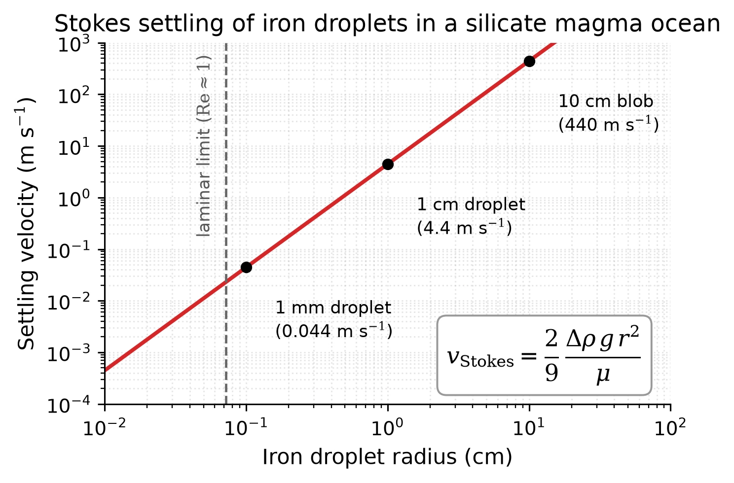
Fig. 4.1 Stokes settling velocity for an iron droplet in a low-viscosity silicate magma ocean as a function of droplet radius (Eq. (4.1)), assuming \(\Delta\rho = 4000\) kg m\(^{-3}\), \(g = 5\) m s\(^{-2}\), and \(\mu = 0.1\) Pa s. The Stokes curve gives \(\sim 4\) m s\(^{-1}\) for centimetre-sized droplets; submillimetre droplets are far slower and are more likely to remain suspended by convection. The dashed vertical line marks the laminar limit (Reynolds number \(\mathrm{Re} \approx 1\), where \(\mathrm{Re}\) compares inertial to viscous forces in the flow; near \(r \approx 0.7\) mm): to its right the flow around the droplet is turbulent and the Stokes curve is an upper bound, with centimetre droplets actually settling at roughly \(0.5\) m s\(^{-1}\) [Rubie et al., 2003], so a 1000 km magma ocean is crossed within weeks rather than days. The strong \(r^2\) dependence is the central reason that iron-silicate separation is geologically instantaneous once droplets coalesce [Rubie et al., 2015]. Course-original figure.

4.1.2. The Moon-forming giant impact

The Moon-forming giant impact occurred when a Mars-sized body struck proto-Earth 4.5 billion years ago. This formed the Moon (Fig. 4.2) [Kegerreis et al., 2022] and completed Earth’s differentiation (Fig. 4.3).

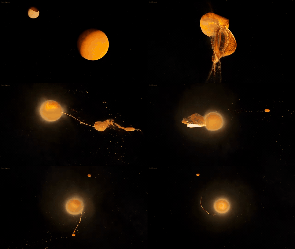
Fig. 4.2 Smoothed-particle hydrodynamics (SPH) simulation of the Moon-forming giant impact, in which a Mars-sized body (Theia) strikes the proto-Earth. The collision ejects long tidal arms of mantle material; part of the debris recollapses onto Earth while an outer clump survives as a satellite on a wide orbit. The animation is strongly time-accelerated. Simulation and visualisation by J. Kegerreis; see Kegerreis et al. [2022].

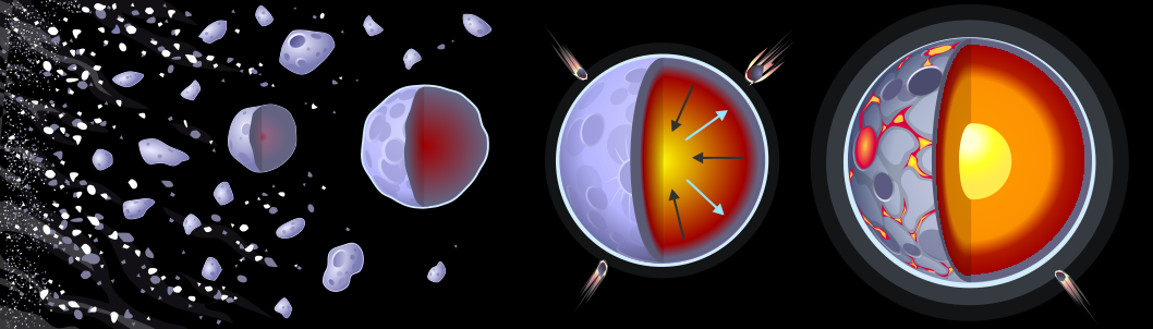
Fig. 4.3 Differentiation of a terrestrial planet. Initially homogeneous accreted material (left) melts due to accretional and radiogenic heating, allowing dense metallic iron to sink and form a core while lighter silicates rise to form the mantle and crust (right). This process occurs rapidly once widespread melting begins. Credit: Wikimedia Commons, CC BY-SA 4.0.

4.1.3. Giant impacts and mantle stripping

For oblique, high-velocity collisions, a giant impact can remove more silicate mantle than it delivers. This mantle stripping leaves a remnant with an anomalously large metallic core relative to its silicate mantle. It explains Mercury’s high iron fraction and provides a model for Mars’s hemispheric dichotomy.

Mercury has a metallic core mass fraction of \(\sim 74\%\) [Margot et al., 2018] (see Lecture 8 and Lecture 10), compared to \(\sim 32\%\) for Earth and \(\sim 24\%\) for Mars. Condensation chemistry alone cannot produce this high iron fraction. The leading hypothesis, going back to Benz et al. [1988] and updated with smoothed-particle hydrodynamics simulations by Benz et al. [2007] and Chau et al. [2018], is a mantle-stripping giant impact: an oblique collision that removed most of the silicate mantle into heliocentric orbit while leaving the metallic core intact (Fig. 4.4).

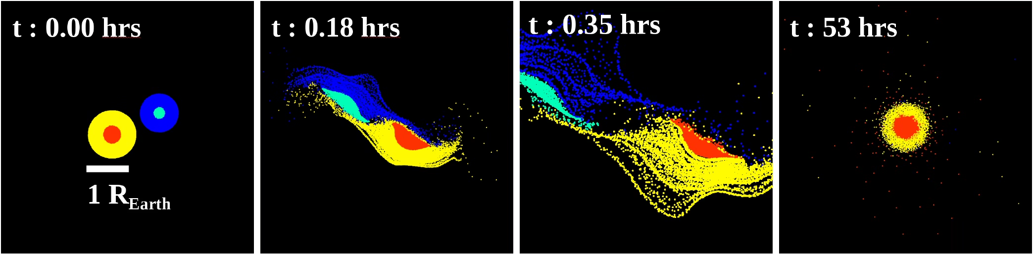
Fig. 4.4 Smoothed-particle hydrodynamics (SPH) simulation of a mantle-stripping giant impact on proto-Mercury from Chau et al. [2018] (their Case 1). A proto-Mercury of 2.25 present Mercury masses (red: core; yellow: mantle) collides with an impactor of half its mass (turquoise: core; blue: mantle) at an impact parameter \(b = 0.5\) and \(v = 30\) km s\(^{-1}\); the white bar marks \(1\,R_\oplus\). The collision preferentially ejects silicate mantle material, and the metal-rich remnant recollapses: after 53 hours the largest fragment holds \(0.95\) of Mercury’s present mass with an iron mass fraction \(Z_\mathrm{Fe} = 0.67\), matching Mercury’s anomalously large core. Snapshots are shown in the \(x\)-\(y\) plane, viewed from above. Reproduced from Chau et al. [2018].

The hemispheric dichotomy of Mars (Lecture 10) is the \(\sim 6\) km elevation and \(\sim 30\) km crustal-thickness difference between the northern lowlands and southern highlands (Fig. 4.5). Andrews-Hanna et al. [2008] and Marinova et al. [2008] proposed that a giant impact excavated the northern hemisphere to produce this dichotomy. Unlike the Mercury collision, this impact redistributed crust laterally rather than stripping mantle mass to space.

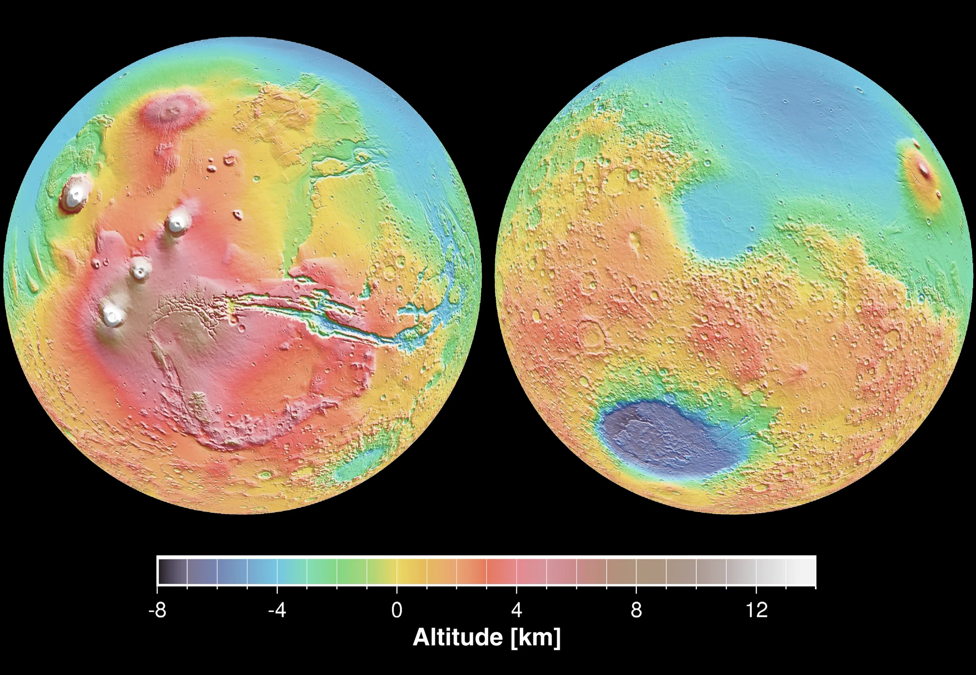
Fig. 4.5 Global false-colour topography of Mars from the Mars Orbiter Laser Altimeter (MOLA) on Mars Global Surveyor, in two orthographic views. The hemispheric dichotomy stands out as the contrast between the smooth, low northern plains (blue) and the ancient, heavily cratered southern highlands (orange to red). The left view also shows the Tharsis volcanic rise (white peaks, including Olympus Mons) and the Valles Marineris canyon system; the deep blue basin in the right view is Hellas. Credit: NASA/JPL, image PIA02820.

The Moon-forming impact represents the opposite regime of net accretion, where a Mars-sized body struck Earth and contributed the material that assembled the Moon. Mercury and Earth represent the endpoints from net mantle stripping to net accretion, while Mars is an intermediate case that redistributed crust without stripping bulk mantle.

Mantle stripping also explains why Mercury’s surface is depleted in iron and sulfur relative to chondrites, primitive meteorites that never melted and preserve solar-nebula composition. The required impact velocities also constrain giant-planet migration during terrestrial-planet assembly (Lecture 2).

4.2. Core formation

The chemical consequences of core formation are profound: the separation of metal from silicate partitions the elements between the core and mantle (an element is said to partition between two coexisting phases when it distributes itself between them in a concentration ratio set by chemical equilibrium), according to their geochemical affinities.

4.2.1. Goldschmidt classification

Elements are classified into four geochemical categories based on phase affinity:

Classification	Affinity	Examples
Siderophile (“iron-loving”)	Metallic phase (core)	Fe, Ni
Lithophile (“rock-loving”)	Silicate phase (mantle)	Si, Mg
Chalcophile (“sulfur-loving”)	Sulfide phase	Cu, S
Atmophile (“atmosphere-loving”)	Gas phase	H, N

This classification (Fig. 4.6) depends on pressure, temperature, and oxygen fugacity (an effective oxygen partial pressure measuring how oxidising or reducing a melt is) during metal-silicate equilibration. At high pressures, silicon becomes siderophile and enters the core, contributing to its density deficit relative to pure iron [Rubie et al., 2015, Shahar et al., 2026].

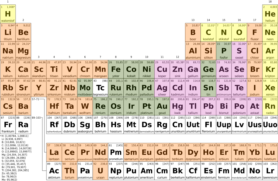
Fig. 4.6 Periodic table coloured by Goldschmidt classification: siderophile (iron-loving), lithophile (rock-loving), chalcophile (sulfur-loving), and atmophile (atmosphere-loving) elements. The classification reflects the preferential partitioning of elements during core-mantle differentiation. Credit: Wikimedia Commons, CC BY-SA 3.0.

4.2.2. Partition coefficients

The degree to which an element partitions into metal is quantified by the metal-silicate partition coefficient:

(4.2)\[ D_i^{\mathrm{met/sil}} = \frac{C_i^{\mathrm{metal}}}{C_i^{\mathrm{silicate}}} \]

Here \(C_i^{\mathrm{metal}}\) and \(C_i^{\mathrm{silicate}}\) are element concentrations in the metallic and silicate phases. Strongly siderophile elements have \(D^{\mathrm{met/sil}} \sim 10^4\) to \(10^6\), concentrating overwhelmingly in the core. The depletion of mantle iridium by a factor of \(\sim 1000\) relative to chondrites provides direct evidence for core formation [Rubie et al., 2015].

However, mantle siderophile elements sit near \(10^{-3}\) of chondritic abundance in chondritic proportions, higher than core formation predicts. This excess is explained by a late veneer, a final \(\sim 0.5\%\) of planetary mass accreted from chondritic material after core formation ceased (Fig. 4.9) [Walker, 2009]. Smaller late veneers are inferred for Mars and the Moon.

Partition coefficients depend strongly on pressure, temperature, and oxygen fugacity (\(f_{\mathrm{O_2}}\)). High pressures at the base of a deep magma ocean (40 to 60 GPa) alter partitioning, allowing laboratory experiments to constrain core-formation conditions.

4.2.3. Equilibration depth and the P-T-\(f_{\mathrm{O_2}}\) dependence

As metal droplets sink through a magma ocean, siderophile element partitioning between core and mantle is determined by the \((P, T, f_{\mathrm{O_2}})\) conditions at the base of the magma ocean [Rubie et al., 2015]. Partition coefficients follow an empirical Nernst-type regression, a thermodynamic parameterisation fit to laboratory experiments:

(4.3)\[ \log_{10} D_i^{\mathrm{met/sil}} = a_i + \frac{b_i}{T} + c_i \frac{P}{T} + d_i \cdot \log_{10} f_{\mathrm{O_2}} \]

For moderately siderophile elements such as Ni and Co, \(D_i^{\mathrm{met/sil}}\) decreases with pressure from \(\sim 10^4\) at 1 GPa to \(\sim 10^2\) or less at 50 GPa. Earth’s mantle retains several percent of its nickel, whereas low-pressure partitioning (\(D \sim 10^3\) to \(10^4\)) predicts near-total depletion. Reproducing observed mantle abundances (\(D \approx 24\) to \(26\) for Ni and Co) requires equilibration at 40 to 60 GPa and 3000 to 4000 K, corresponding to a magma ocean \(\sim 1000\) to \(1500\) km deep (Fig. 4.7) [Fischer et al., 2015].

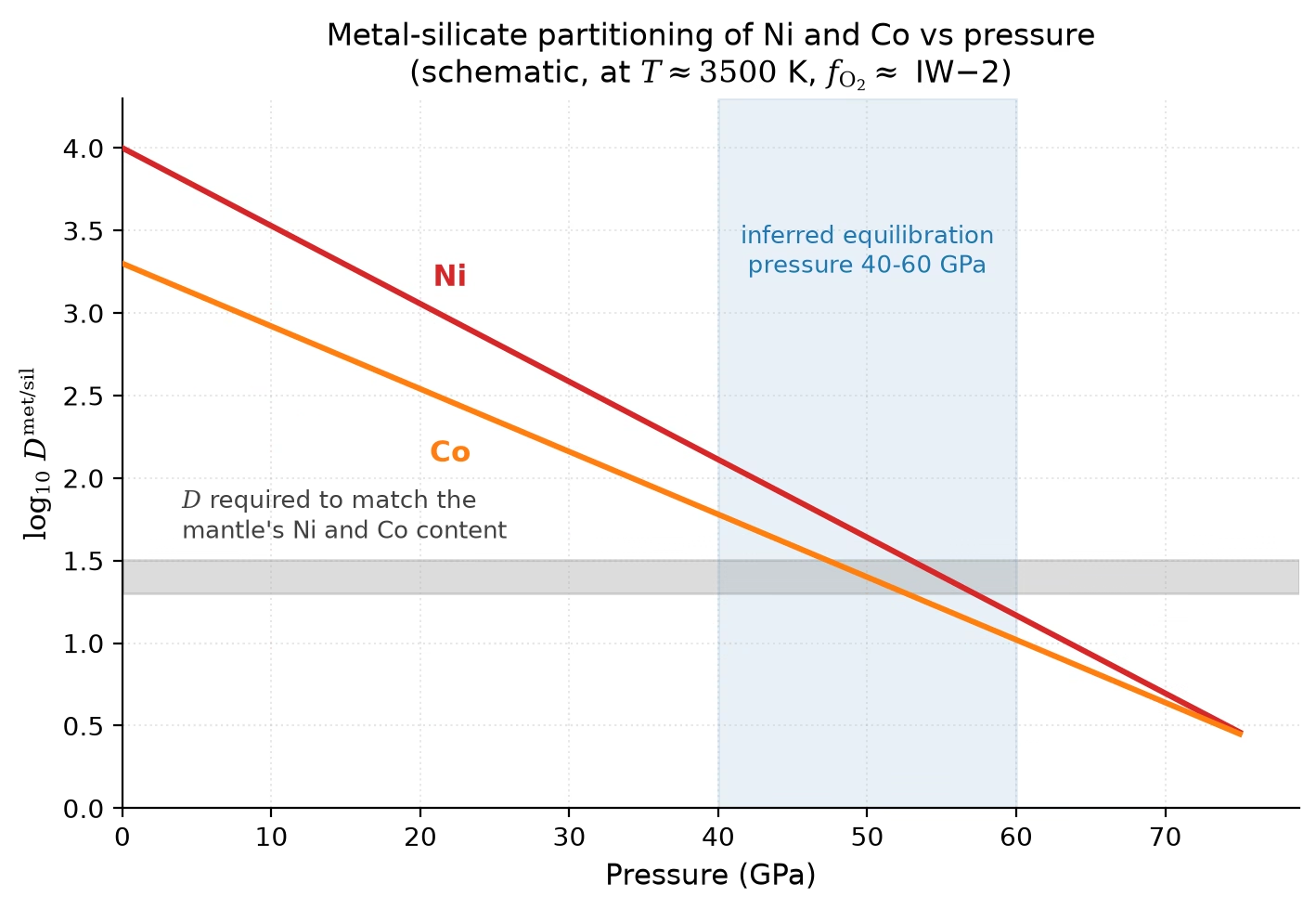
Fig. 4.7 Pressure dependence of the metal-silicate partition coefficients of nickel and cobalt (schematic; the lines follow Eq. (4.3) at fixed \(T \approx 3500\) K and \(f_{\mathrm{O_2}} \approx\) IW\(-\)2). At low pressure both elements partition very strongly into the metal (\(D \sim 10^3\)–\(10^4\)), which would strip the mantle of Ni and Co almost completely. The horizontal grey band marks the \(D\) values that reproduce the Ni and Co content actually observed in Earth’s mantle (\(D_\mathrm{Ni} \approx 26\), \(D_\mathrm{Co} \approx 24\) from core-mantle mass balance). The measured partition coefficients fall to these values only at pressures near \(40\)–\(60\) GPa (blue band): the experiments of Fischer et al. [2015] place single-stage equilibration at \(54 \pm 5\) GPa and 3300–3400 K, at the base of a \(\sim 1000\)–\(1500\) km deep magma ocean. Schematic redrawn after the experimental results of Siebert et al. [2013] and Fischer et al. [2015]; see also Rubie et al. [2015]. Course-original figure.

The oxygen fugacity \(f_{\mathrm{O_2}}\) measures the chemical availability of oxygen, represented as the effective partial pressure of \(\mathrm{O_2}\) in equilibrium with the melt. In a reducing environment (low \(f_{\mathrm{O_2}}\)) iron remains metallic, while in an oxidising environment (high \(f_{\mathrm{O_2}}\)) iron oxidises to FeO and enters the silicate. Values are quoted relative to the iron-wüstite (IW) buffer, \(\mathrm{Fe} + \tfrac{1}{2}\mathrm{O_2} \rightleftharpoons \mathrm{FeO}\), with IW\(-\)2 indicating 2 orders of magnitude below reference. During accretion, \(f_{\mathrm{O_2}}\) rose from 4 to 5 log-units below IW to near IW\(-\)2 today. Increasing oxygen availability oxidises more metal into the silicate, lowering \(D_i^{\mathrm{met/sil}}\) and reproducing mantle abundances in a progressively oxidising magma ocean [Rubie et al., 2015].

Core formation proceeds continuously during accretion rather than as an instantaneous event. The two-stage Hf-W model age of \(\sim 30\) Myr compresses core extraction into an equivalent single event, setting a lower limit on core completion [Kleine and Walker, 2017]. Because accretion was protracted, Earth’s core finished forming after \(\sim 30\) Myr, mostly within \(\sim 100\) Myr and no later than 200 Myr. In contrast to this planetary timescale, individual metal droplets equilibrated with the magma ocean in only days (Fig. 4.1).

4.2.4. Hf-W chronometry: timing core formation

The hafnium-tungsten (Hf-W) isotopic system dates core formation via the decay of short-lived \({}^{182}\mathrm{Hf}\) to \({}^{182}\mathrm{W}\) (half-life 8.9 million years). Hafnium is lithophile (stays in the mantle) while tungsten is moderately siderophile (extracted into the core). Early core formation while \({}^{182}\mathrm{Hf}\) is alive produces an excess of mantle \({}^{182}\mathrm{W}\) relative to undifferentiated chondrites (Fig. 4.8), whereas late core formation leaves no excess.

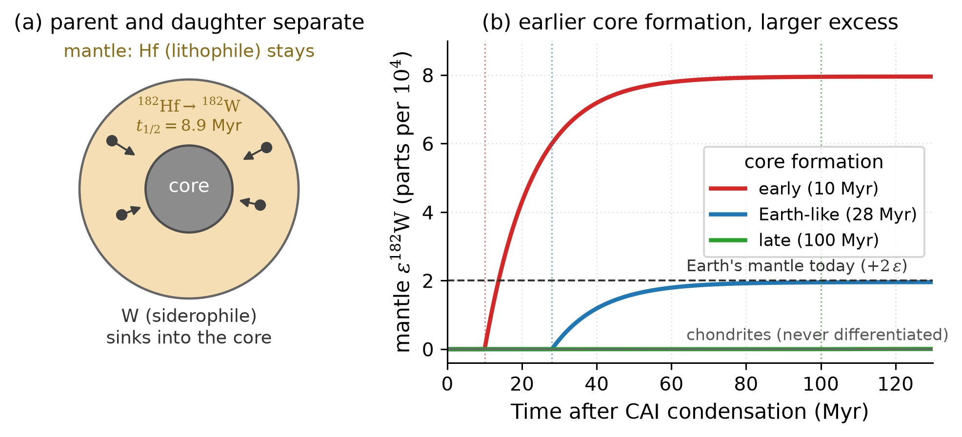
Fig. 4.8 How Hf-W chronometry dates core formation. (a) Core formation separates the parent from the daughter reservoir: hafnium is lithophile and stays in the mantle, where \({}^{182}\mathrm{Hf}\) keeps decaying to \({}^{182}\mathrm{W}\) (\(t_{1/2} = 8.9\) Myr), while tungsten is siderophile and sinks into the core with the metal. (b) Resulting mantle \({}^{182}\mathrm{W}\) excess for core formation at three different times, computed from the two-stage model of Eq. (4.4) with Earth’s mantle Hf/W enrichment. Early core formation leaves much live \({}^{182}\mathrm{Hf}\) in the mantle and builds a large excess; core formation after \({}^{182}\mathrm{Hf}\) is extinct leaves none. Earth’s measured excess of \(+2\) \(\varepsilon\)-units corresponds to a two-stage age of \(\sim 28\) Myr. The excess also scales with the mantle’s Hf/W enrichment, which differs between bodies; this is why Mars shows a smaller excess than Earth despite forming its core earlier. See Kleine et al. [2009]. Course-original figure.

The mantle \({}^{182}\mathrm{W}\) excess, expressed as \(\varepsilon^{182}\mathrm{W}\) in parts per 10,000 deviation from chondritic, records the timing of core formation. For Earth, \(\varepsilon^{182}\mathrm{W} \approx +2\) yields a two-stage model age of \(\sim 30\) Myr, a lower limit for protracted accretion that was mostly complete within \(\sim 100\) Myr [Kleine and Walker, 2017]. For Mars, bulk-mantle \(\varepsilon^{182}\mathrm{W} \approx +0.37 \pm 0.05\), estimated from enriched shergottites (a class of basaltic martian meteorites), indicates accretion within \(\sim 10\) Myr [Kruijer et al., 2017]. The Moon’s \(\varepsilon^{182}\mathrm{W}\) is close to Earth’s value, consistent with formation from giant impact debris.

Core-formation timing across the solar system is summarised in Fig. 4.9. The zero point (\(t = 0\)) is defined by CAIs (calcium-aluminium-rich inclusions, the first solids to condense from the solar nebula). Meteoritic records of the first 5 Myr are covered in Lecture 12, while Fig. 4.9b compares core formation across planetesimals, Mars, Earth, and the Moon.

4.2.4.1. Worked example: from \(\varepsilon^{182}\mathrm{W}\) to a core-formation age

In a two-stage model, core formation occurs instantaneously at time \(t_c\) after CAIs (\(t = 0\)). Metal segregation removes tungsten into the core, elevating mantle \(\mathrm{Hf/W}\). Decay of residual \(^{182}\mathrm{Hf}\) produces an excess of \(^{182}\mathrm{W}\) in the mantle:

(4.4)\[ \varepsilon^{182}\mathrm{W}_\mathrm{BSE} = \mathcal{Q}_\mathrm{W} \cdot \left[\frac{(\mathrm{Hf}/\mathrm{W})_\mathrm{BSE}}{(\mathrm{Hf}/\mathrm{W})_\mathrm{CHUR}} - 1\right] \cdot \left(\frac{{}^{182}\mathrm{Hf}}{{}^{180}\mathrm{Hf}}\right)_{\!\!\!0} \cdot e^{-\lambda t_c} \]

where \(\mathcal{Q}_\mathrm{W} \approx 10^4\) is the prefactor, \((^{182}\mathrm{Hf}/^{180}\mathrm{Hf})_0 \approx 1.02 \times 10^{-4}\) is the initial ratio, \(\lambda = 7.79 \times 10^{-2}\ \mathrm{Myr}^{-1}\) is the decay constant (\(t_{1/2} = 8.9\) Myr), and CHUR (chondritic uniform reservoir) denotes unfractionated composition. For Earth’s bulk silicate mantle (\(\mathrm{BSE}\)), \((\mathrm{Hf}/\mathrm{W})_\mathrm{BSE}/(\mathrm{Hf}/\mathrm{W})_\mathrm{CHUR} \approx 18\), so the bracketed term is \(\approx 17\).

Plugging in the observed Earth value \(\varepsilon^{182}\mathrm{W}_\mathrm{BSE} \approx +2\):

\[ e^{-\lambda t_c} = \frac{2}{10^4 \cdot 17 \cdot 1.02 \times 10^{-4}} \approx 0.115 \]

\[ t_c = -\frac{\ln 0.115}{\lambda} \approx \frac{2.16}{0.0779\ \mathrm{Myr}^{-1}} \approx 28 \text{ Myr} \]

For Earth, this yields an instantaneous age of \(\sim 28\) Myr. Protracted accretion makes this a lower limit, with core formation extending to \(\sim 100\) Myr [Kleine and Walker, 2017]. For Mars, \((\mathrm{Hf}/\mathrm{W})_\mathrm{mantle}/(\mathrm{Hf}/\mathrm{W})_\mathrm{CHUR} \approx 4\) and \(\varepsilon^{182}\mathrm{W} \approx +0.4\) yield a model age of \(\sim 26\) Myr. Since martian core formation ended within \(\sim 10\) Myr (Fig. 4.9), this signature dates magma-ocean crystallisation at \(\sim 20\) to \(25\) Myr [Kruijer et al., 2017]. Mars thus accreted and differentiated before \(^{182}\mathrm{Hf}\) became extinct.

The Hf-W system only dates processes occurring while \(^{182}\mathrm{Hf}\) is alive, within \(\sim 45\) Myr of CAIs. Later differentiation leaves no \(\varepsilon^{182}\mathrm{W}\) signature, so events such as inner core nucleation require thermal-evolution modelling (Lecture 8).

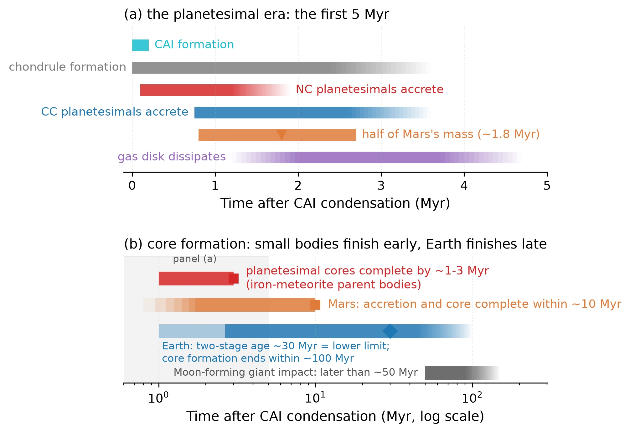
Fig. 4.9 Chronology of accretion and core formation, in time after CAI condensation. (a) The planetesimal era on a linear axis: CAIs condense at \(t = 0\); chondrules form and non-carbonaceous (NC) and carbonaceous (CC) planetesimals accrete over the first \(\sim 4\) Myr; Mars reaches half of its final mass at \(\sim 1.8\) Myr; the gas disk dissipates within \(\sim 5\) Myr. Spans are schematic, redrawn after Fig. 4 of Lichtenberg et al. [2023] and references therein. (b) Core formation on a logarithmic axis: planetesimal cores, sampled by the iron meteorites, are complete by \(\sim 1\)–\(3\) Myr; Mars finishes its accretion and core formation within \(\sim 10\) Myr [Kleine and Walker, 2017, Kruijer et al., 2017]; Earth’s two-stage Hf–W age of \(\sim 30\) Myr (diamond) is a lower limit, with core formation ending within \(\sim 100\) Myr; the Moon-forming giant impact occurs later than \(\sim 50\) Myr [Kleine and Walker, 2017, Nimmo and Kleine, 2015]. Fading bar ends indicate uncertain boundaries. Course-original figure.

4.3. Mantle differentiation

Core formation is not the end of chemical differentiation. As the magma ocean cools and crystallises, it produces further chemical layering within the silicate mantle itself.

4.3.1. Magma ocean crystallisation

As a magma ocean cools, solidification begins where its adiabat (the temperature profile of a convecting fluid with depth) meets the melting curves of peridotite (mantle rock). Below the solidus the mantle is solid, above the liquidus it is liquid, and between them crystals and melt form a mush. Because melting curves rise more steeply with pressure than the adiabat, cooling crosses the liquidus first at the base of the mantle (Fig. 4.10). A deep magma ocean therefore crystallises from the bottom up [Elkins-Tanton, 2012], forming high-pressure bridgmanite (\(\mathrm{MgSiO_3}\)) at depth and olivine at shallower depths.

Solidification displaces liquid upward, enriching remaining melt in incompatible elements (U, Th, K, and rare earths). The final stages leave a buoyant residual liquid enriched in volatiles and heat-producing elements at the top of the mantle.

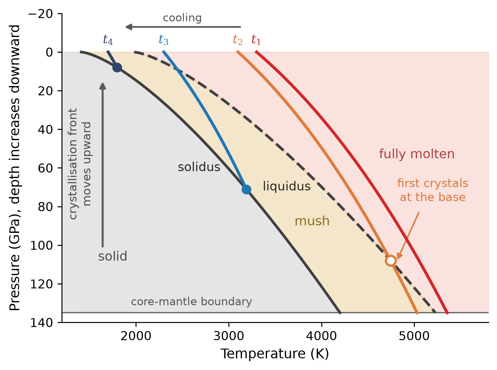
Fig. 4.10 Why a deep magma ocean crystallises from the bottom up. The solidus (solid black curve) and liquidus (dashed black curve) of peridotite are shown together with magma-ocean adiabats at successive times \(t_1\) to \(t_4\) as the planet cools; each adiabat is drawn down to the depth where it meets the solidus, below which the mantle is solid. Because the melting curves rise more steeply with pressure than the adiabats, a cooling adiabat first drops below the liquidus at the base of the mantle (\(t_2\), open circle): the first crystals appear at depth. Between the solidus and the liquidus, crystals and melt coexist as a mush. At later times the adiabat–solidus intersection (filled circles), the crystallisation front, sits at progressively shallower depth. Curves are schematic for an Earth-sized mantle, after the melting-curve and adiabat systematics reviewed by Elkins-Tanton [2012]. Course-original figure.

At lowermost-mantle pressures, the density contrast between melt and crystals shrinks, allowing iron-rich melt to become denser than solids. This dense melt can persist as a long-lived basal magma ocean [Labrosse et al., 2007]. InSight seismology indicates a molten silicate layer above the core-mantle boundary of Mars [Samuel et al., 2023].

4.3.2. Incompatible element enrichment

During crystallisation, incompatible elements that do not fit into mineral crystal lattices concentrate in the residual liquid. These include the heat-producing isotopes uranium (U), thorium (Th), and potassium (K) (Lecture 3).

The residual liquid solidifies to form the crust. Continental crust is enriched in U, Th, and K by a factor of \(\sim\)50–100 relative to the upper mantle, producing roughly half of Earth’s radiogenic heat in less than 1% of Earth’s mass.

4.3.3. Mantle reservoirs

The crystallisation of a magma ocean does not produce a perfectly homogeneous mantle. Instead, it creates compositionally distinct mantle reservoirs that persist to the present day:

• Depleted MORB mantle (DMM): The upper mantle source of mid-ocean ridge basalts (MORBs) has been depleted in incompatible elements by billions of years of partial melting and crustal extraction. This is the most voluminous mantle reservoir.

• Enriched mantle: Deep mantle plumes that produce ocean island basalts (OIBs, e.g., Hawaii, Iceland) sample reservoirs that are enriched in incompatible elements, possibly representing less-processed primordial mantle material or recycled oceanic crust.

Fig. 4.11 summarises the reservoirs and the two transfers that link them.

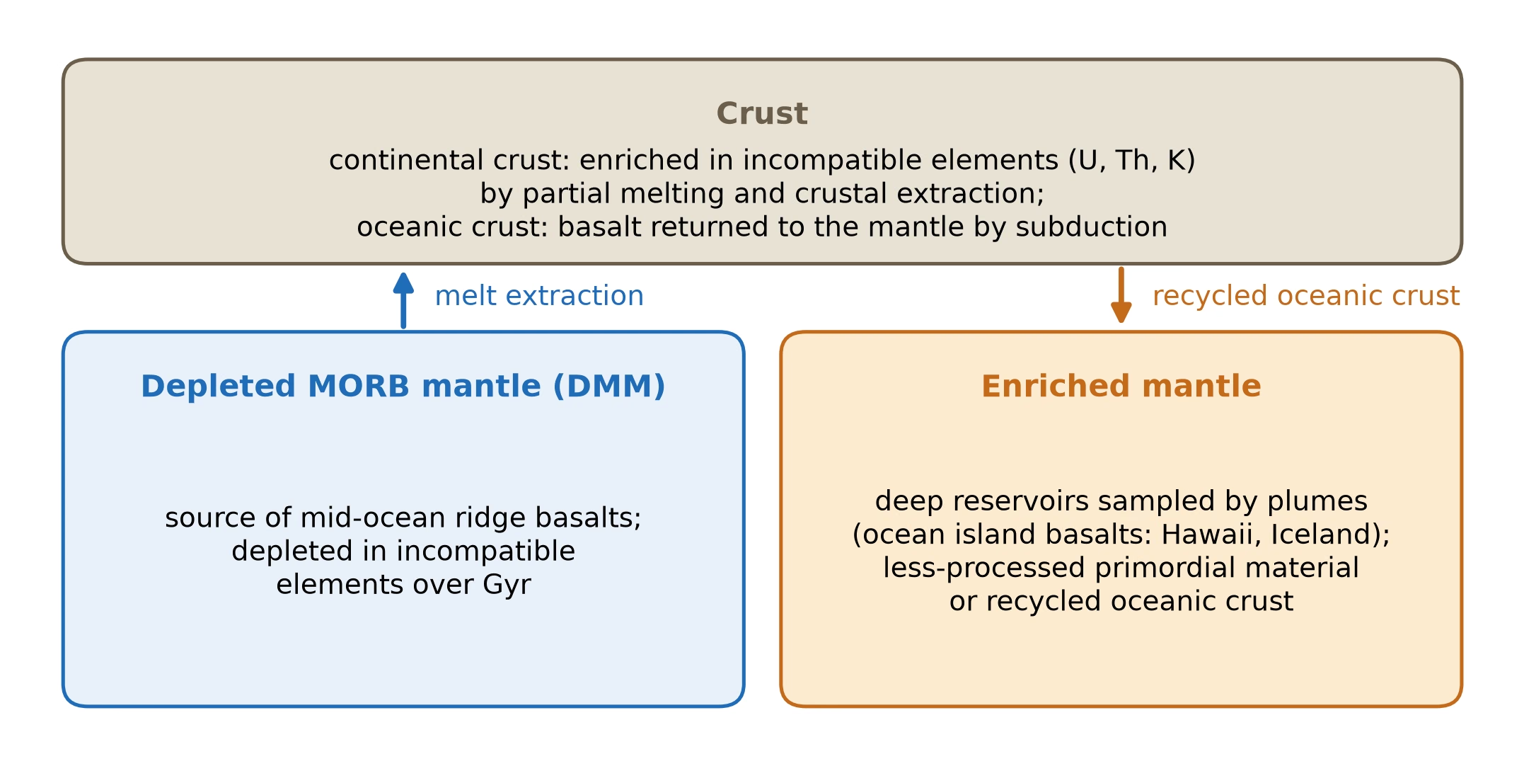
Fig. 4.11 Mantle reservoirs left by magma ocean crystallisation and by later melting. The depleted MORB mantle, the source of mid-ocean ridge basalts, lost its incompatible elements to the continental crust over billions of years of partial melting; oceanic crust returns to the mantle by subduction. The enriched mantle sampled by plumes, the source of ocean island basalts, holds primordial material or recycled oceanic crust. Schematic. Course-original figure.

4.3.4. The lunar magma ocean

The Moon provides the clearest example of magma ocean crystallisation. Apollo 11 returned fragments of white anorthosite (rock made almost entirely of plagioclase feldspar) from Mare Tranquillitatis in 1969. To explain a global plagioclase crust, Wood et al. [1970] proposed that buoyant plagioclase crystals floated to the surface of a deep magma ocean.

Because of its small size and single-plate tectonic regime, the Moon has largely preserved this magma-ocean stratigraphy (Fig. 4.12). Beneath the \(\sim 40\) to \(50\) km anorthositic crust lies a cumulate mantle (rock built from crystals that settled out of the magma) grading from pyroxenite to dunite. The last residual liquid crystallised at the base of the crust into a layer enriched in dense ilmenite and KREEP (potassium, rare earth elements, and phosphorus), which is thought to have sunk through the underlying mantle in an early gravitational overturn [Elkins-Tanton, 2012].

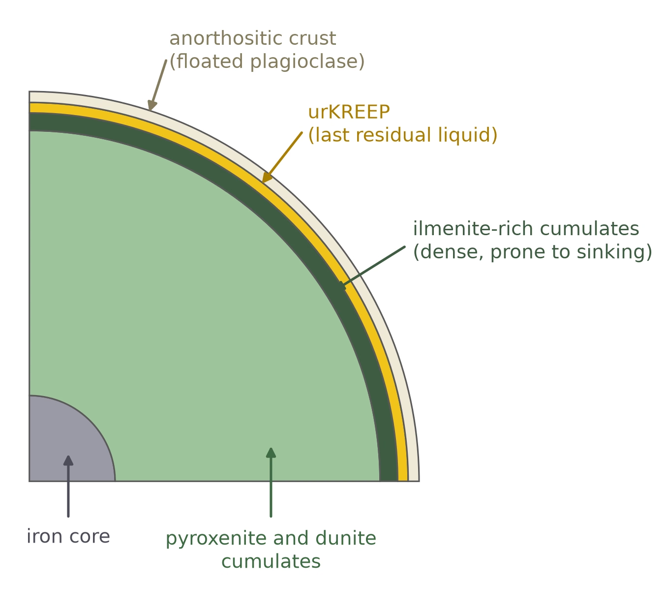
Fig. 4.12 Section cutout of the Moon at the end of magma-ocean solidification. The outer \(\sim 40\)–\(50\) km is the anorthositic crust (pale), formed by flotation of plagioclase on top of the crystallising magma ocean. Directly beneath it, the thin urKREEP layer (yellow) is the last \(\sim 1\%\) of the original magma ocean to solidify and is concentrated in incompatible trace elements, including the heat-producing isotopes \(^{40}\mathrm{K}\), \(^{235,238}\mathrm{U}\), and \(^{232}\mathrm{Th}\). The dense ilmenite-rich cumulates (dark green) formed near the end of crystallisation just below the urKREEP layer; they are gravitationally unstable and sank toward the core, driving the lunar mantle overturn that dominated lunar tectonics in the first \(\sim 500\) Myr after crystallisation. The pyroxenite and dunite cumulates (light green) solidified during the intermediate crystallisation stages, and an iron core sits at the centre. The thicknesses of the crust, urKREEP, and ilmenite layers are exaggerated for visibility. Stratigraphy after Elkins-Tanton [2012]. Course-original figure.

This flotation crust forms the bright highlands visible on the lunar nearside (Fig. 4.13). The dark maria are thin sheets of basaltic lava that flooded large impact basins hundreds of millions of years after the magma ocean solidified.

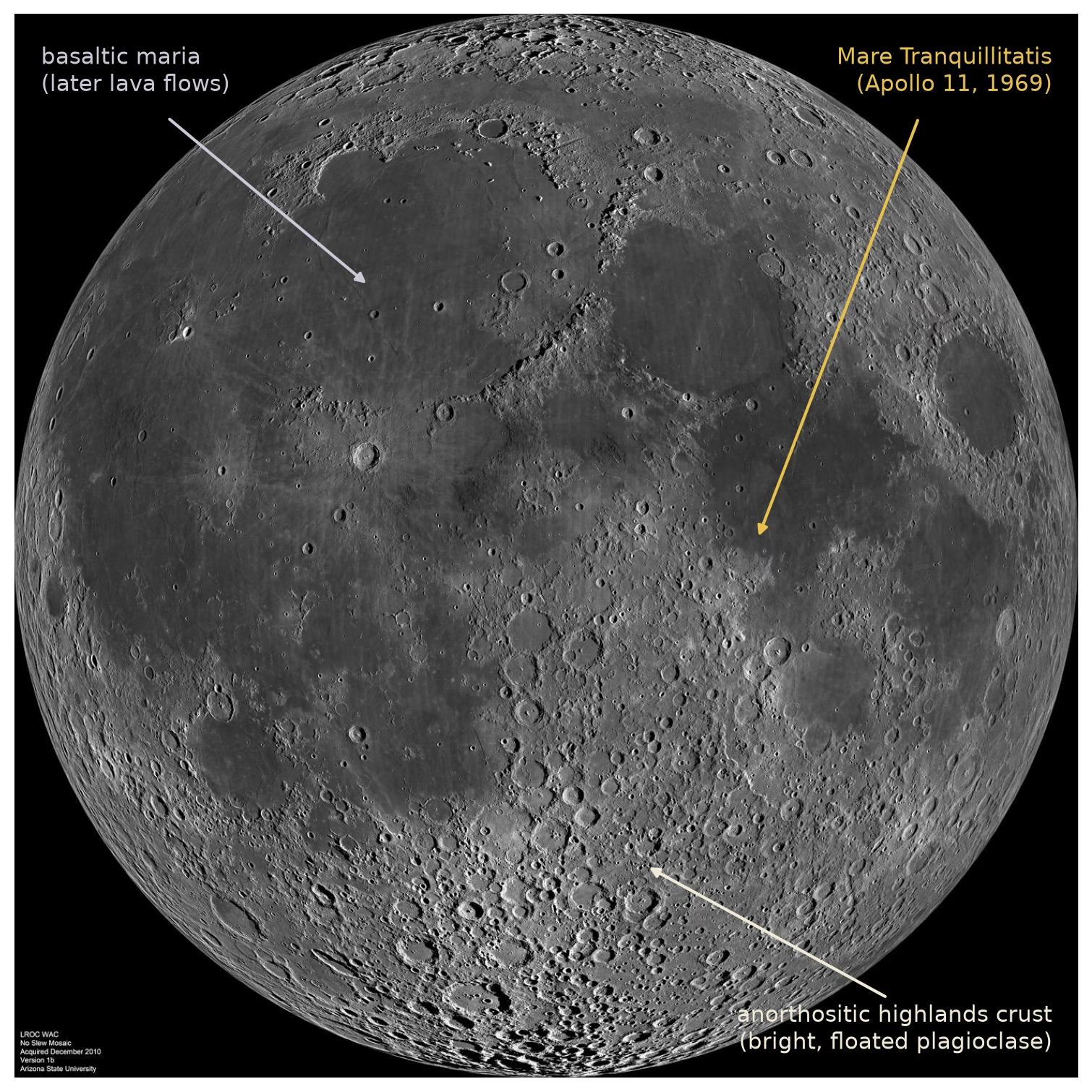
Fig. 4.13 The lunar nearside as a direct view of magma-ocean stratigraphy. The bright, heavily cratered highlands are the anorthositic flotation crust of the lunar magma ocean; the dark maria are later basaltic lava flows that flooded the major impact basins. The Apollo 11 landing site at the south-western edge of Mare Tranquillitatis is where the first anorthosite fragments were collected in 1969, leading Wood et al. [1970] to propose the magma ocean concept. Lunar Reconnaissance Orbiter Camera wide-angle mosaic. Credit: NASA/GSFC/Arizona State University (PIA14011), public domain; annotations added for this course.

4.4. Volatile delivery and retention

The chemical differentiation discussed so far concerns the refractory (high-temperature) components of planets. But the volatile elements (hydrogen, carbon, nitrogen, sulfur, and the noble gases) are equally important, because they form the raw materials for atmospheres, oceans, and ultimately life.

4.4.1. The classical view and its revision

In the classical view, terrestrial planets formed inside the snow line (the distance from the Sun beyond which water condenses as ice, at \(\sim\)2–3 AU) from dry rock. Water and other volatiles were thought to arrive late, delivered by asteroids and comets scattered inward after the planets had finished growing (Fig. 4.14a).

Meteorite measurements demonstrate that the inner solar system was never completely dry. All chondrite groups, including ordinary and enstatite chondrites from the inner disk, accreted water ice during their formation [Alexander, 2019]. Because the snow line migrated outward during peak accretional heating and then retreated inward as the disk cooled, early inner planetesimals accreted ice directly [Grewal et al., 2024].

As Jupiter grew, it dammed the inward drift of icy pebbles and split the disk into two distinct planetesimal reservoirs (Fig. 4.14b). This division produced the isotopically distinct non-carbonaceous (NC) and carbonaceous (CC) meteorite families. Isotopic measurements of nitrogen, carbon, and sulfur indicate that Earth accreted volatiles from both reservoirs during its main growth rather than from a late veneer [Grewal et al., 2021].

Although inner building blocks incorporated ice, terrestrial planets are dry today, with Earth’s surface water amounting to only a few hundredths of a percent of its mass. Growing protoplanets lost most of this water during accretion through three main mechanisms [Lichtenberg et al., 2023].

First, decay heat from \(^{26}\)Al melted early planetesimals and drove off their ice (Lecture 3), leaving dry, differentiated bodies [Lichtenberg et al., 2019]. Second, impact devolatilisation (the escape of vaporised species during collisions) removed volatiles and moderately volatile elements like magnesium during giant impacts [Hin et al., 2017].

Third, infalling icy pebbles ablated in primordial hydrogen envelopes, recycling water vapour into the disk rather than delivering it to the surface [Johansen et al., 2021]. A planet’s final volatile budget is therefore set early by the timing of planetesimal and giant planet formation, and trimmed during accretion by radiogenic heating, collisional loss, and atmospheric processing [Krijt et al., 2023].

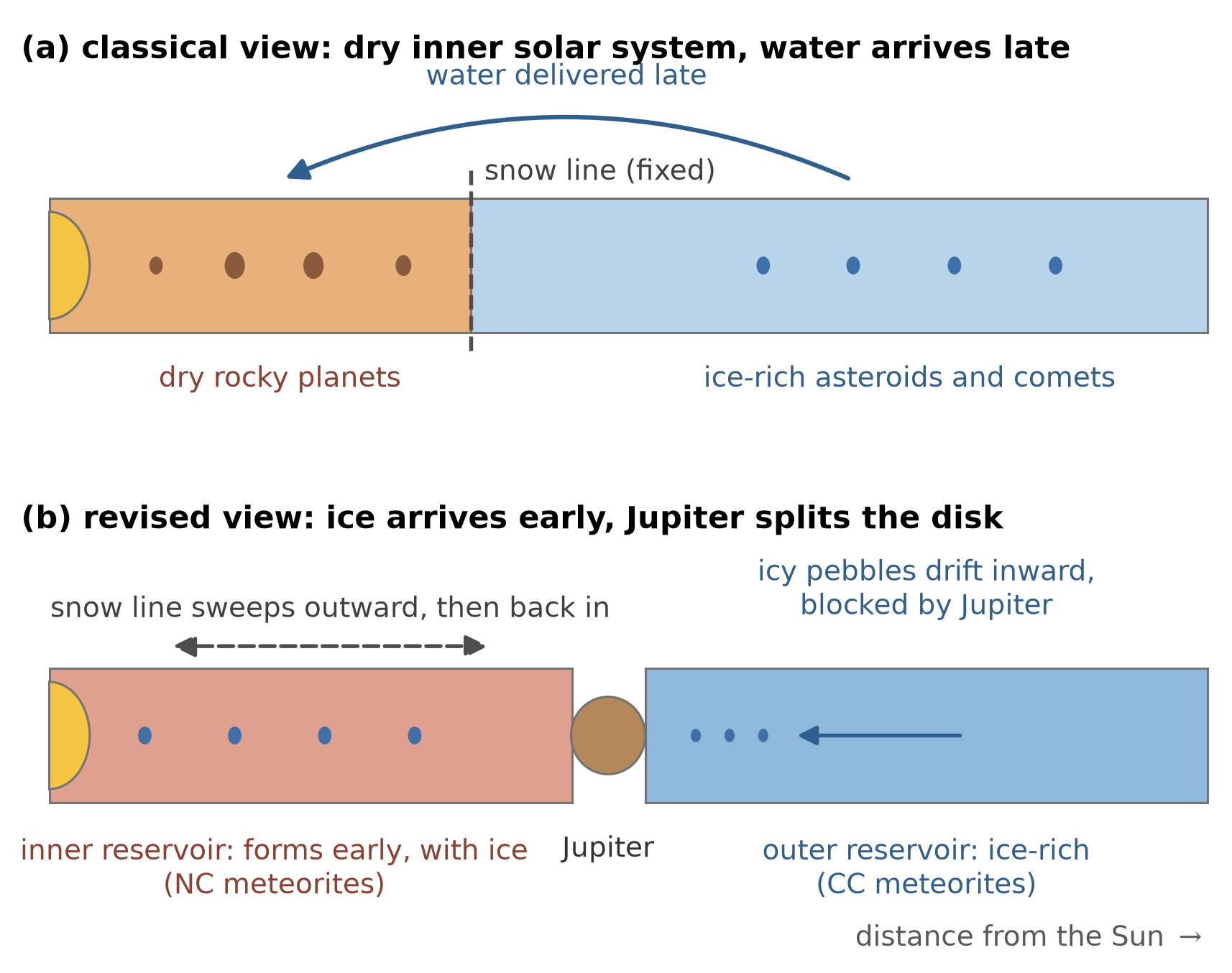
Fig. 4.14 Volatile delivery to the terrestrial planets: the classical and the revised picture. (a) In the classical view a fixed snow line separates a dry inner disk from an ice-rich outer disk, and water reaches the finished terrestrial planets late, through asteroids and comets scattered inward. (b) In the revised view the snow line first sweeps outward through the young disk and then retreats inward as the disk cools, so the earliest inner planetesimals form beyond it and accrete ice (blue bodies in the inner reservoir); Jupiter’s growth then blocks the inward drift of icy pebbles, splitting the disk into an inner and an outer reservoir. These two reservoirs correspond to the NC and CC meteorite families [Alexander, 2019, Grewal et al., 2024, Lichtenberg et al., 2021]. Course-original figure.

4.4.2. Outgassing from the magma ocean

Much of a planet’s initial volatile budget is dissolved in the silicate magma ocean. As the magma ocean cools and crystallises, dissolved volatiles are released to form a secondary atmosphere through outgassing [Hirschmann, 2012].

Atmospheric speciation depends on the oxygen fugacity of the magma:

• Under reducing conditions (low \(f_{\mathrm{O_2}}\)): dominant species are \(\mathrm{H_2}\), CO, and \(\mathrm{N_2}\)

• Under oxidising conditions (high \(f_{\mathrm{O_2}}\)): dominant species are \(\mathrm{H_2O}\), \(\mathrm{CO_2}\), and \(\mathrm{N_2}\)

Volatile partitioning between melt and atmosphere is set by gas solubility in silicate melt. Water dissolves as hydroxyl groups, whereas \(\mathrm{CO_2}\) forms carbonate ions and is roughly two orders of magnitude less soluble. Because dissolving water splits into two hydroxyl groups, the dissolved water fraction grows with the square root of vapour pressure:

(4.5)\[ X_{\mathrm{H_2O}} \propto p_{\mathrm{H_2O}}^{1/2} \]

where \(X_{\mathrm{H_2O}}\) is the mole fraction of dissolved water and \(p_{\mathrm{H_2O}}\) is the vapour pressure above the melt. This feedback allows the magma ocean to retain more water in solution as the atmosphere thickens [Hirschmann, 2012].

Most of a planet’s water thus remains in the magma during the magma ocean stage (Fig. 4.15) [Nicholls et al., 2024]. Across most oxidation states, Earth’s mantle melt holds \(\sim 5 \times 10^{21}\) kg of water (over 3 times the ocean mass) while the atmosphere contains only a few bar of steam. Poorly soluble carbon instead dominates the atmosphere as \(\mathrm{CO_2}\) and CO at hundreds to thousands of bar.

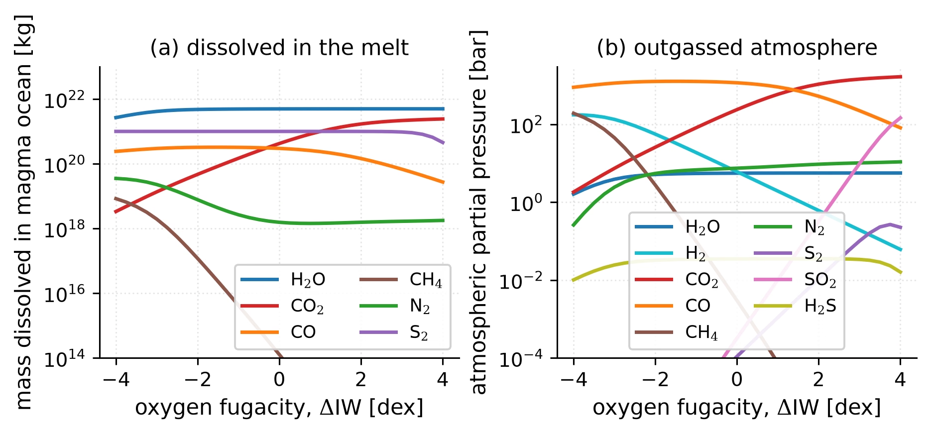
Fig. 4.15 Equilibrium partitioning of Earth’s volatile inventory between a fully molten magma ocean and its outgassed atmosphere, as a function of the melt oxygen fugacity (expressed as the logarithmic shift \(\Delta\)IW relative to the iron-wüstite buffer), computed with an equilibrium outgassing model [Nicholls et al., 2024] for the bulk silicate Earth H/C/N/S inventory of Krijt et al. [2023] and a mantle temperature of 2000 K. (a) Mass of each volatile species dissolved in the melt. The dissolved water mass is nearly constant at \(\sim 5 \times 10^{21}\) kg, more than 3 times the mass of the present-day ocean: the melt retains nearly the whole water inventory at all but the most reducing conditions. (b) Partial pressures in the atmosphere. Carbon species dominate throughout (CO on the reduced side, CO\(_2\) on the oxidised side) because carbon is far less soluble in the melt than water; the steam partial pressure never exceeds a few bar. Under reducing conditions H\(_2\) and CH\(_4\) take over from CO\(_2\); at the most oxidised end SO\(_2\) rises steeply. Course-original figure.

4.4.3. Impact erosion versus delivery

Giant impacts deliver volatiles but can also strip them away. Impact erosion (atmospheric loss driven by collisions) operates in two distinct regimes depending on impactor size.

In local erosion, an impactor vaporises upon impact, driving a plume that accelerates overlying gas beyond escape velocity. A single impact removes at most the atmosphere above the plane tangent to the surface [Melosh and Vickery, 1989]. For a thin atmosphere (\(H \ll R\)), the tangent-plane fraction is

(4.6)\[ f_\mathrm{tp} \approx \frac{H}{2R} \]

about \(6 \times 10^{-4}\) of the global inventory for Earth (\(H \approx 8\) km). Because a single impact removes little gas, local erosion operates through cumulative bombardment. Small planetesimals are the most efficient eroders per unit mass because their energy couples directly into the atmosphere [Schlichting et al., 2015].

In global erosion, a giant impact sends a shock through the interior that sets the ground into motion. Wherever ground velocity satisfies

(4.7)\[ v_\mathrm{ground} \gtrsim v_\mathrm{esc}, \]

the overlying atmospheric column is expelled. In the Moon-forming impact, ground velocities remained well below Earth’s \(v_\mathrm{esc} \approx 11\) km s\(^{-1}\), removing only \(\sim 20\%\) of the atmosphere [Genda and Abe, 2003]. However, a surface ocean enhances loss because water vaporisation and lower shock impedance (the product of density and wave speed) transmit ground motion more efficiently [Genda and Abe, 2005]. This ocean effect may explain why dry Venus retains roughly 50 times more \(^{36}\mathrm{Ar}\) than Earth.

Three-dimensional simulations resolve two distinct channels within a single event (Fig. 4.16): near-field loss from ejecta plumes, and far-field loss from global shock breakout [Roche et al., 2025]. Atmospheric loss ranges from a few percent in oblique collisions near escape velocity to near-total removal in high-velocity head-on impacts.

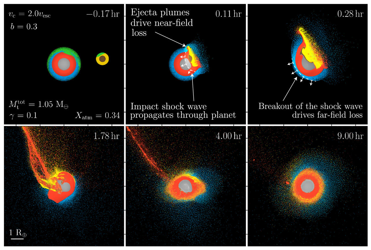
Fig. 4.16 Atmospheric loss during a giant impact, in snapshots from a smoothed-particle hydrodynamics simulation of a moderately oblique collision (impact parameter \(b = 0.3\)) between a \(1.05\,M_\oplus\) planet carrying a primordial H\(_2\)-He envelope and an impactor holding one tenth of the total colliding mass, striking at twice the mutual escape velocity. Particles are coloured by material: target core (grey), target mantle (orange), atmosphere (blue), impactor core (brown), and impactor mantle (yellow); particles that become unbound and are lost from the planet are coloured green. Near the impact site, ejecta plumes drive near-field loss; the impact shock (white dashed line) travels through the planet, breaks out at the surface, and drives far-field loss over the rest of the globe. In this event 34% of the atmosphere is lost. Figure 1 of Roche et al. [2025], CC BY 4.0.

Earth’s primordial H\(_2\)-He envelope was stripped by cumulative impacts alongside solar XUV-driven thermal escape (Lecture 5). For Mars, with lower escape velocity (\(\approx 5\) km s\(^{-1}\)), a Borealis-scale impact (Marinova et al. [2008]) and solar-wind stripping removed most of the early atmosphere (Lecture 10).

Planetary volatile inventories reflect the balance between impact delivery and erosion, set by impactor size, velocity, and volatile content [Schlichting et al., 2015]. Earth’s volatile budget combines this balance with secondary outgassing from the magma ocean.

The evolution of outgassed atmospheres is discussed in Lecture 5 and Lecture 6.

4.5. Planetary magnetic fields and dynamo theory

The differentiation of a planet into a metallic core and silicate mantle sets the stage for one of the most important geophysical phenomena: the generation of a planetary magnetic field by dynamo action in the liquid metallic core.

4.5.1. Why magnetic fields matter

A global magnetic field deflects charged solar wind particles, reducing surface radiation and atmospheric erosion. This limits sputtering (atmospheric atoms knocked loose by energetic particles) and ion pickup (ionised particles swept away by the solar wind). Mars lost much of its atmosphere after losing its global field \(\sim\)4 Gyr ago (Lecture 10).

Magnetic minerals record the ambient field when cooling through their Curie temperature (the temperature above which a mineral loses its permanent magnetism). The field also provides direct constraints on the physical state, composition, and dynamics of a planet’s deep interior.

Fig. 4.17 contrasts a shielded and an unshielded planet.

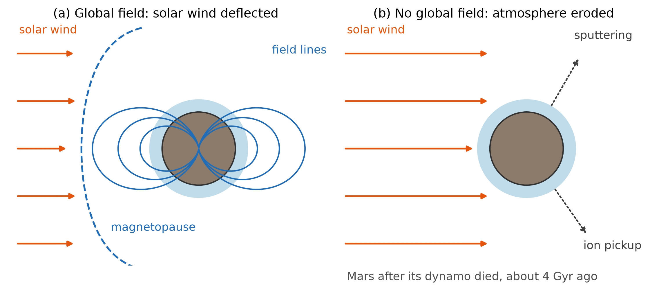
Fig. 4.17 A global magnetic field as a shield for the atmosphere. (a) A magnetised planet: the solar wind is held off at the magnetopause, and the upper atmosphere lies inside the field lines. (b) An unmagnetised planet: the solar wind reaches the upper atmosphere directly, neutral atoms leave by sputtering and ions by pickup, the fate of Mars after its dynamo died about 4 Gyr ago. Schematic, not to scale. Course-original figure.

4.5.2. The induction equation

The magnetic induction equation describes magnetic field evolution in a conducting fluid:

(4.8)\[ \pdv{\vec{B}}{t} = \nabla \times (\vec{v} \times \vec{B}) + \eta \nabla^2 \vec{B} \]

where \(\vec{B}\) is magnetic field, \(\vec{v}\) is fluid velocity, and \(\eta\) is magnetic diffusivity:

(4.9)\[ \eta = \frac{1}{\mu_0 \sigma} \]

with permeability \(\mu_0 = 4\pi \times 10^{-7}\) H m\(^{-1}\) and electrical conductivity \(\sigma\).

Two competing terms govern field survival [Roberts and King, 2013]. Advection \(\nabla \times (\vec{v} \times \vec{B})\) stretches field lines to amplify magnetic flux. Diffusion \(\eta \nabla^2 \vec{B}\) causes ohmic decay that destroys flux.

4.5.3. Requirements for dynamo action

A self-sustaining dynamo generates and maintains a magnetic field against ohmic decay when three conditions are met:

1. An electrically conducting fluid to carry currents (liquid iron in terrestrial planets, metallic hydrogen in gas giants).

2. Convection driven by thermal or compositional buoyancy.

3. Flow vigour where advection dominates diffusion, requiring the magnetic Reynolds number \(\mathrm{Rm}\) to exceed \(\mathrm{Rm}_c \sim 10\) to \(100\).

Convective columns aligned with the rotation axis stretch and twist field lines to regenerate the field (Fig. 4.18).

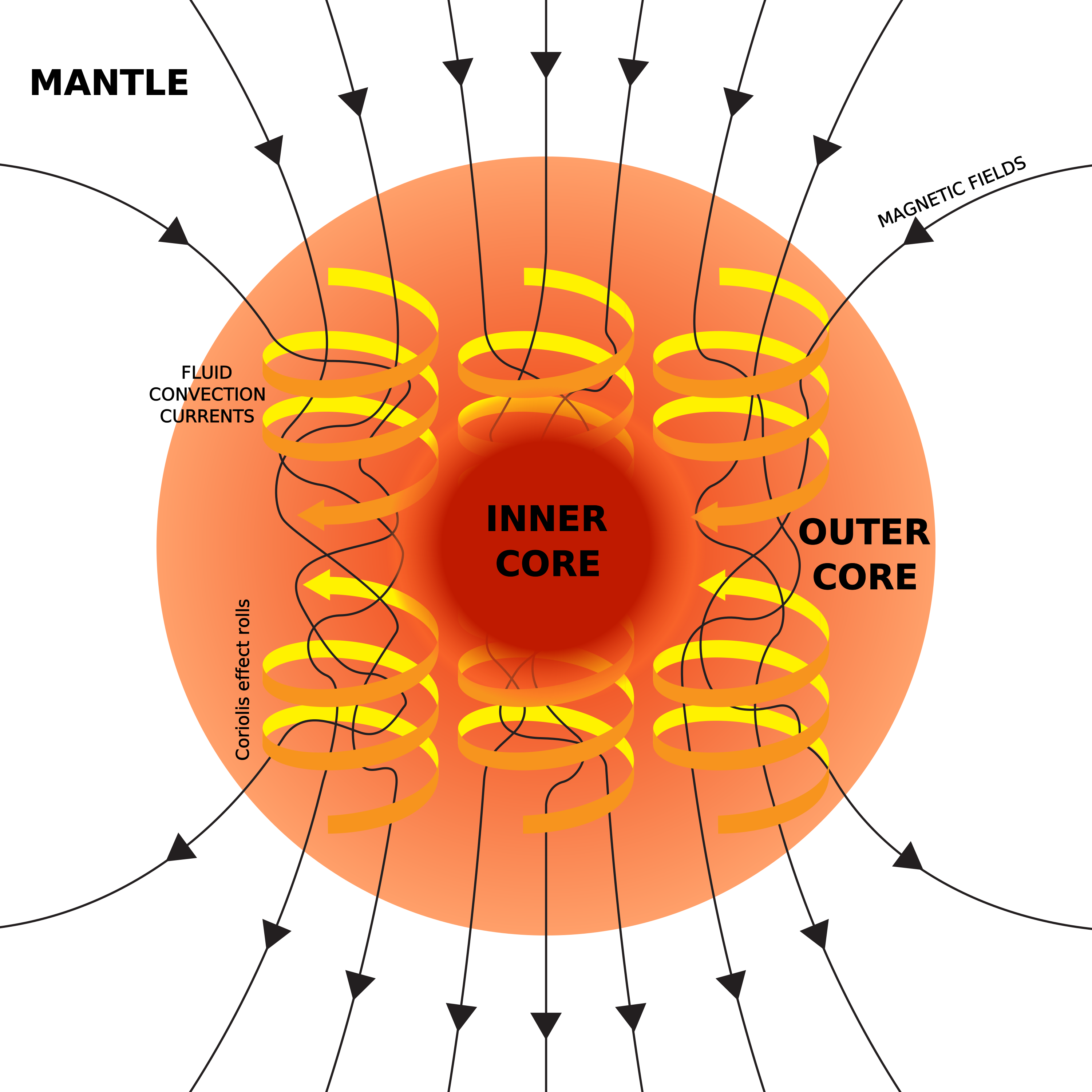
Fig. 4.18 Schematic of the geodynamo mechanism. Convective motions in the electrically conducting liquid outer core stretch and twist magnetic field lines, generating Earth’s predominantly dipolar magnetic field. The Coriolis force organises the flow into columnar structures aligned with the rotation axis. Credit: Wikimedia Commons, CC BY-SA 4.0.

Fig. 4.19 shows the two terms of the induction equation and, for Earth’s outer core, how far \(\mathrm{Rm}\) exceeds the critical value.

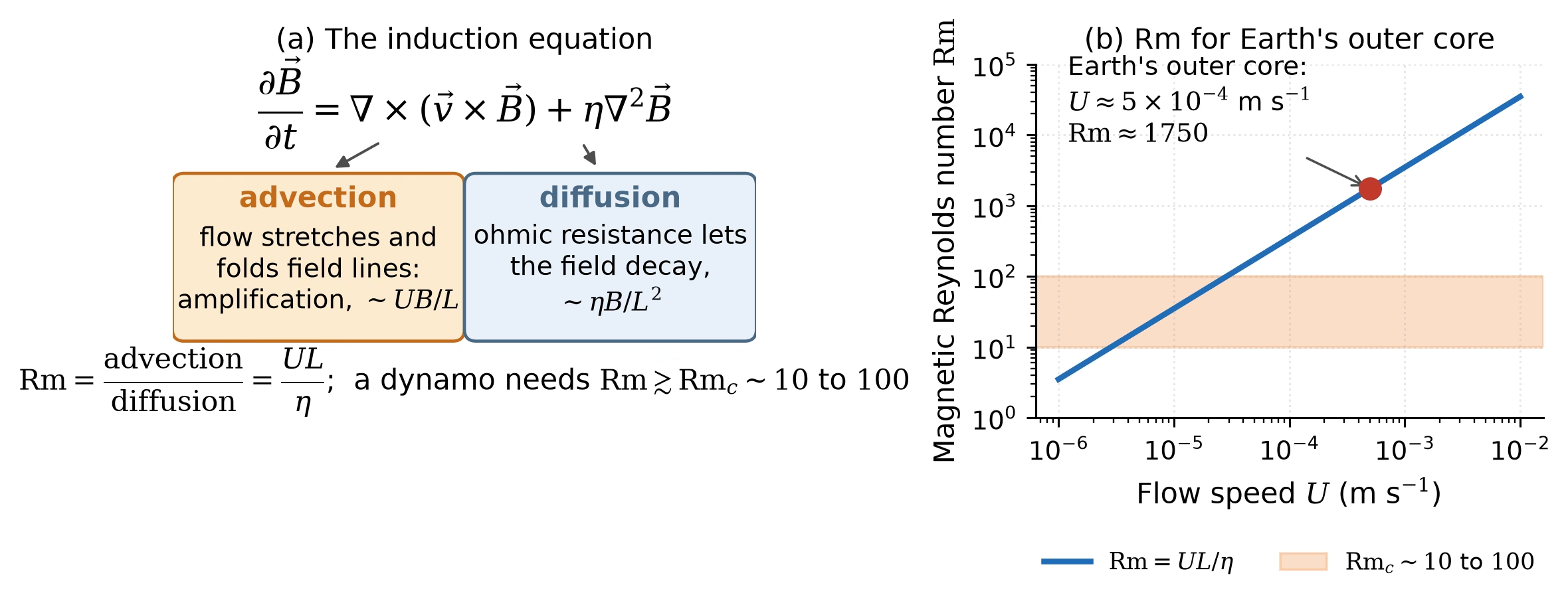
Fig. 4.19 The induction equation and the magnetic Reynolds number. (a) The advection term stretches and folds field lines and amplifies the field at a rate of order \(UB/L\); the diffusion term lets the field decay at a rate of order \(\eta B/L^2\); their ratio is \(\mathrm{Rm} = UL/\eta\), and a dynamo needs \(\mathrm{Rm}\) above a critical value of order 10 to 100. (b) \(\mathrm{Rm}\) for Earth’s outer core against the flow speed, with \(L = 3.5 \times 10^6\) m and \(\eta = 1\) m\(^2\) s\(^{-1}\): at \(U \approx 5 \times 10^{-4}\) m s\(^{-1}\) the estimate is about 1750, far above the critical range. Course-original figure.

4.6. Blackboard derivation: The magnetic Reynolds number

Blackboard derivation: The magnetic Reynolds number \(\mathrm{Rm}\)

Goal: Derive the magnetic Reynolds number \(\mathrm{Rm} = UL/\eta\) from the induction equation by dimensional analysis, and estimate \(\mathrm{Rm}\) for Earth’s outer core to demonstrate that advection dominates over diffusion, the fundamental criterion for dynamo action.

Setup.

We start from the magnetic induction equation introduced in the previous section (Eq. (4.8)):

\[ \pdv{\vec{B}}{t} = \underbrace{\nabla \times (\vec{v} \times \vec{B})}_{\text{advection}} + \underbrace{\eta \nabla^2 \vec{B}}_{\text{diffusion}} \]

We want to determine which term dominates for a given flow. If advection wins, the flow can amplify magnetic field; if diffusion wins, any field decays away.

Fig. 4.20 shows the setup: a conducting fluid shell of thickness \(L\) moves with speed \(U\) around the inner core and threads the field \(\vec{B}\).

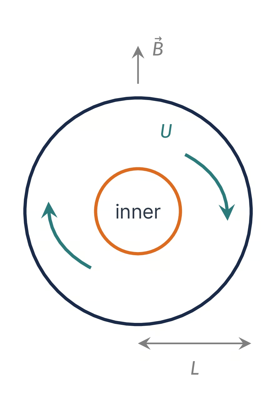
Fig. 4.20 Setup sketch of the board derivation of the magnetic Reynolds number: the outer core as a conducting fluid shell of size \(L\) around the inner core, with flow speed \(U\) and the magnetic field \(\vec{B}\) that the flow advects and diffusion erodes. Course-original figure.

Derivation.

We use dimensional analysis to estimate the magnitude of each term. Let \(U\) be a characteristic flow velocity, \(L\) a characteristic length scale, and \(B\) the field strength.

Advection term:

\[ |\nabla \times (\vec{v} \times \vec{B})| \sim \frac{UB}{L} \]

since the curl introduces a factor of \(1/L\) and the cross product introduces a factor of \(UB\).

Diffusion term:

\[ |\eta \nabla^2 \vec{B}| \sim \frac{\eta B}{L^2} \]

since each spatial derivative introduces a factor of \(1/L\), and \(\nabla^2\) involves two spatial derivatives.

The ratio of the advection term to the diffusion term defines the magnetic Reynolds number:

\[ \mathrm{Rm} = \frac{|{\text{advection}}|}{|{\text{diffusion}}|} = \frac{UB/L}{\eta B/L^2} \]

Notice that the magnetic field strength \(B\) cancels: this is an important result. The magnetic Reynolds number is a property of the flow, not of the field:

(4.10)\[ \boxed{\mathrm{Rm} = \frac{UL}{\eta}} \]

When \(\mathrm{Rm} \gg 1\), advection dominates: the magnetic field is “frozen in” to the fluid and carried along with the flow. When \(\mathrm{Rm} \ll 1\), diffusion dominates: the field decays regardless of the flow.

For a self-sustaining dynamo, numerical simulations and theory indicate that the critical value is \(\mathrm{Rm}_c \sim 10\)–\(100\), depending on the flow geometry.

Application: Earth’s outer core.

For Earth’s outer core, the relevant parameters are [Schubert et al., 2001]:

Parameter	Symbol	Value
Outer core radius	\(L\)	\(\sim 3.5 \times 10^6\) m
Typical flow velocity	\(U\)	\(\sim 5 \times 10^{-4}\) m s\(^{-1}\)
Magnetic diffusivity	\(\eta\)	\(\sim 1\) m\(^2\) s\(^{-1}\)

This gives:

\[ \mathrm{Rm}_\oplus = \frac{UL}{\eta} = \frac{5 \times 10^{-4} \times 3.5 \times 10^6}{1} \approx 1750 \]

Since \(\mathrm{Rm}_\oplus \approx 1750 \gg \mathrm{Rm}_c\), advection overwhelmingly dominates over diffusion in Earth’s outer core. The flow is vigorous enough to sustain dynamo action.

We can also estimate the ohmic diffusion timescale, how long the field would take to decay if the flow suddenly stopped:

\[ \tau_{\mathrm{ohm}} \sim \frac{L^2}{\eta} = \frac{(3.5 \times 10^6)^2}{1} \approx 1.2 \times 10^{13} \text{ s} \approx 400{,}000 \text{ yr} \]

This is much less than Earth’s age (4.5 Gyr), confirming that the field cannot be a relic; it must be continuously regenerated by dynamo action.

Note: Paleomagnetic measurements of ancient rocks show that Earth has had a magnetic field for at least 3.4–3.5 billion years [Tarduno et al., 2010]. This places a strong constraint on the thermal and compositional evolution of the core: the convective driving mechanism must have been sustained over most of Earth’s history.

4.7. Earth’s geodynamo

With the theoretical framework established, we now examine how the dynamo operates in Earth’s core.

4.7.1. Core structure

Earth’s core comprises a solid inner core (radius 0–1220 km, iron-nickel alloy) and a liquid outer core (radius 1220–3480 km) where the geodynamo operates (Fig. 4.21).

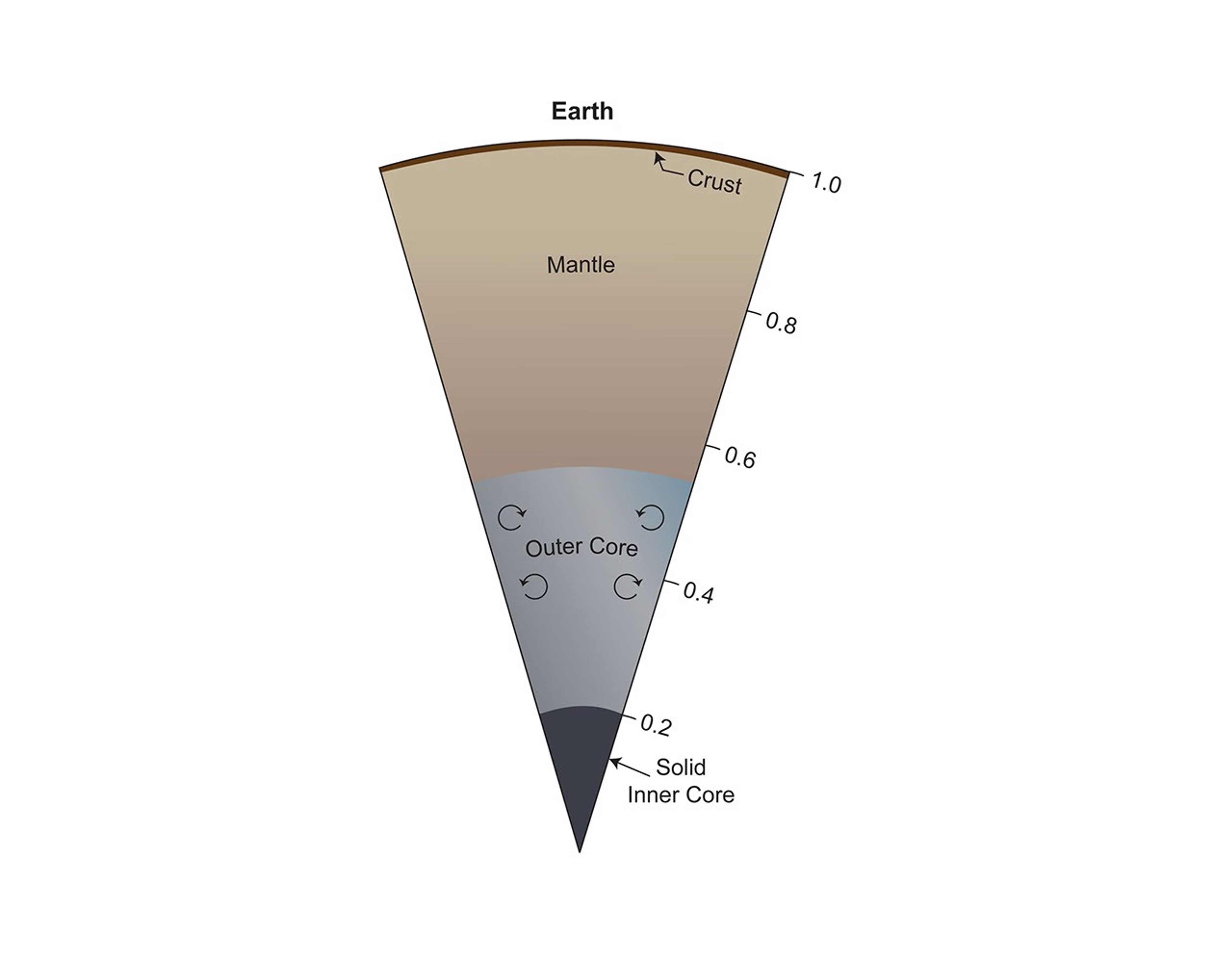
Fig. 4.21 Cross-section of Earth’s interior, showing the solid inner core (\(r < 1220\) km), the liquid iron-alloy outer core (1220 to 3480 km), the silicate mantle (from \(\sim 30\) km depth at the crust base down to 2890 km at the core-mantle boundary), and the thin crust. The geodynamo operates in the convecting outer core; the inner core grows slowly as light elements are expelled into the outer core. Credit: NASA/JPL-Caltech/SwRI/J.E.P. Connerney (PIA25063), public domain.

Seismic \(S\) waves cannot penetrate the liquid outer core (Fig. 4.22) [Oldham, 1906]. Refraction creates a \(P\)-wave shadow zone (103° to 143°), within which weak PKIKP arrivals detect the solid inner core.

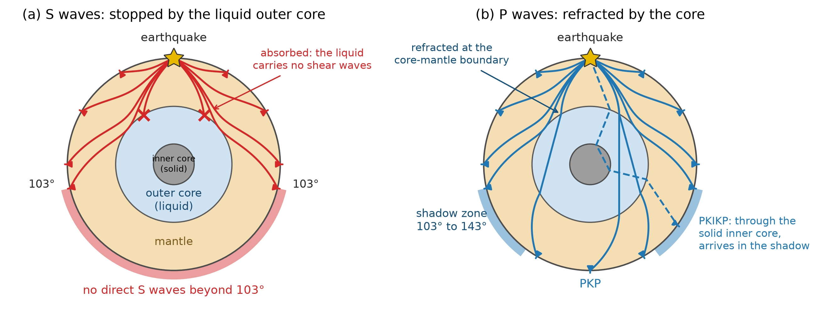
Fig. 4.22 How \(P\) and \(S\) waves constrain the structure of the core. (a) \(S\) waves (red) travel through the solid mantle but stop at the core-mantle boundary because the liquid outer core cannot support shear: no direct \(S\) wave arrives beyond an epicentral distance of about 103°, which shows that the outer core is liquid. (b) \(P\) waves (blue) cross the core but are refracted towards the vertical at the core-mantle boundary, where the \(P\)-wave velocity drops from about 13.7 to 8 km s\(^{-1}\); the refracted rays (PKP) emerge only beyond about 143°, leaving a \(P\)-wave shadow zone between 103° and 143°. Waves refracted a second time through the solid inner core (PKIKP, dashed) arrive inside the shadow zone; their detection revealed the inner core. The phase names spell out the ray path, one letter per leg: P for a compressional leg in the mantle, K for the leg through the liquid outer core, I for the leg through the solid inner core. The shadow-zone argument located the core itself [Oldham, 1906]. Layer radii are to scale; the ray paths are schematic. Course-original figure.

Travel times constrain internal velocity and density profiles in the Preliminary Reference Earth Model (Fig. 4.23) [Dziewonski and Anderson, 1981].

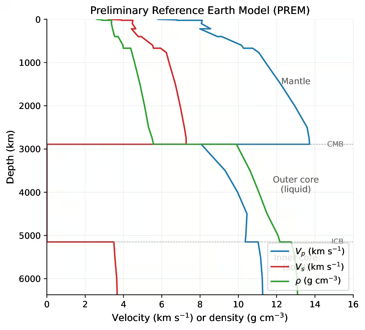
Fig. 4.23 Preliminary Reference Earth Model (PREM) seismic \(P\)-wave velocity (\(V_p\), blue), \(S\)-wave velocity (\(V_s\), red), and density (\(\rho\), green) versus depth. The vanishing \(V_s\) in the outer core (2890–5150 km depth) is direct evidence that this region cannot support transverse elastic waves, i.e. it is liquid; the discontinuous jumps in density at the core-mantle boundary (CMB) and inner-core boundary (ICB) record the metal-silicate interface and the latent heat of inner-core crystallisation respectively. Curve digitised from Dziewonski and Anderson [1981].

4.7.2. Driving mechanisms

Outer core convection is driven by two buoyancy sources [Roberts and King, 2013]. Thermal convection operates when mantle cooling sinks dense fluid, provided heat loss exceeds adiabatic conduction. Compositional convection occurs as inner core crystallisation rejects light elements (S, Si, O).

Inner core growth at about 0.5 mm per year makes compositional buoyancy the dominant geodynamo driver (Fig. 4.24).

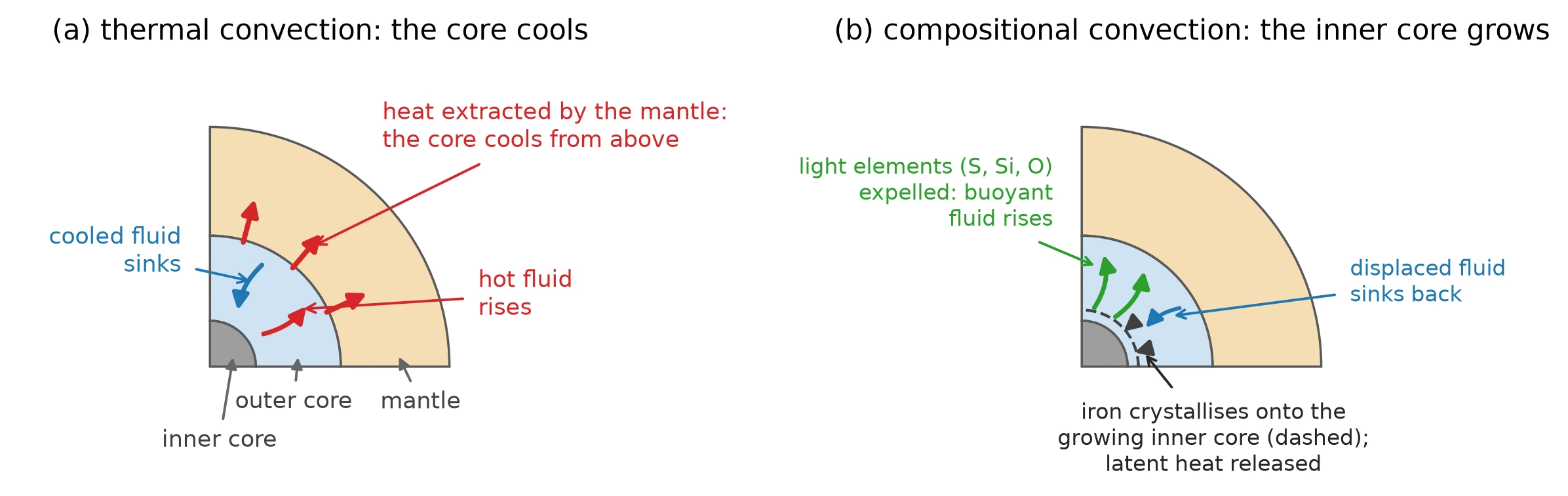
Fig. 4.24 The two buoyancy sources that drive convection in Earth’s liquid outer core, shown in a quarter-section cutout. (a) Thermal convection: the mantle extracts heat across the core-mantle boundary, so the core cools from above; the cooled, dense fluid at the top of the outer core sinks while hot fluid rises from depth. (b) Compositional convection: iron crystallises onto the growing inner core (dashed) and the light elements (S, Si, O) are rejected into the liquid at the inner-core boundary; the buoyant, light-element-enriched fluid rises, displaced fluid sinks back, and the latent heat of crystallisation adds thermal buoyancy. Compositional buoyancy dominates the power budget of the present-day geodynamo [Roberts and King, 2013]. Layer radii are to scale; the flow arrows are schematic. Course-original figure.

4.7.3. Field morphology

Earth’s magnetic field at the surface is predominantly dipolar (resembling the field of a bar magnet), with the dipole axis tilted approximately 11° from the rotation axis. The surface field strength ranges from about 25 \(\mu\)T near the equator to about 65 \(\mu\)T near the poles, with a mean of about 45 \(\mu\)T.

4.7.4. Secular variation

Secular variation is the change in the magnetic field on decadal to century timescales, tracing turbulent outer-core flow. Non-dipole components drift, grow, and decay, with many features exhibiting westward drift at roughly 0.2° per year from differential core-mantle rotation. The South Atlantic Anomaly is a region where the field is about 30% weaker than the global average at that latitude, caused by a reversed-flux patch at the core-mantle boundary.

4.7.5. Polarity reversals

The geomagnetic field undergoes polarity reversals, in which the north and south magnetic poles swap. A reversal takes roughly 1000 to 10,000 years, averaging 4 to 5 reversals per million years.

Magnetic stripes are symmetric patterns of magnetised crust formed at mid-ocean ridges, recording alternating field directions (Fig. 4.25).

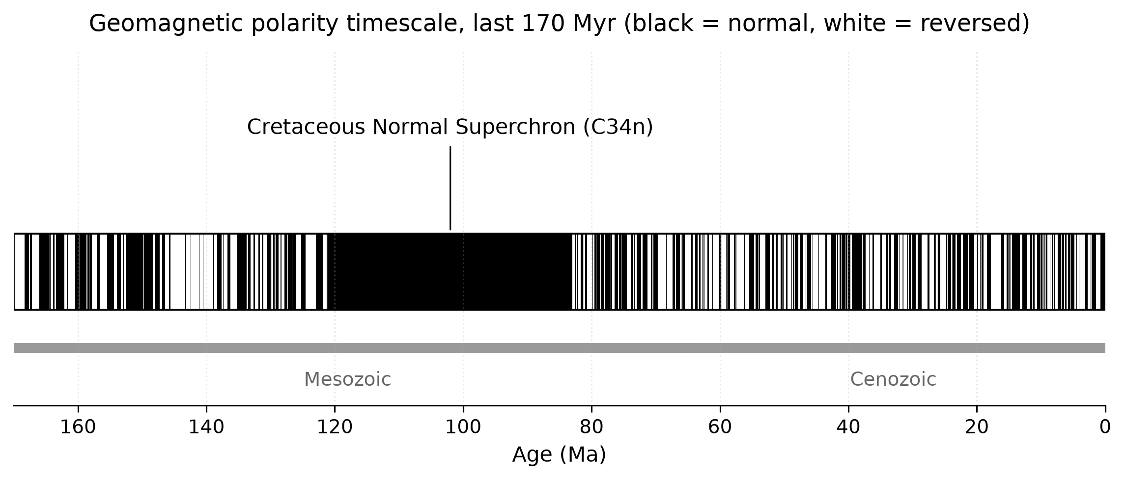
Fig. 4.25 Geomagnetic polarity timescale for the past 170 Myr. Black bars mark intervals of normal polarity (north magnetic pole near the geographic north), white bars mark reversed polarity. The reversal rate has varied from \(\sim 4\)–\(5\) per Myr in the late Cenozoic to essentially zero during the Cretaceous Normal Superchron (CNS, C34n, \(\sim 83\)–\(121\) Ma), shown as the long uninterrupted black band in the middle of the panel. The Mesozoic and Cenozoic era intervals (boundary at \(\sim 66\) Ma) are marked below the axis. Reversals appear statistically consistent with a non-stationary Poisson process, as expected for the chaotic dynamics of the geodynamo. Schematic; boundary ages are approximate and should not be read to better than \(\sim 1\) Myr. Exact chron ages follow the Geologic Time Scale 2020 compilation [Gradstein et al., 2020]. Course-original figure.

4.8. Comparative magnetospheres

Magnetic fields vary enormously across the solar system. Comparing them reveals how dynamo action depends on a planet’s size, composition, thermal state, and rotational dynamics.

4.8.1. Magnetic field comparison

Body	Field type	Dipole moment (relative to Earth)
Earth	Active dynamo	1
Mercury	Active dynamo	\(\sim 5 \times 10^{-4}\)
Venus	None detected	\(< 10^{-5}\)
Mars	Remnant crustal	n/a
Jupiter	Active dynamo	\(\sim 20{,}000\)
Saturn	Active dynamo	~600
Uranus	Active dynamo	~50
Neptune	Active dynamo	~28
Ganymede	Active dynamo	\(\sim 1.5 \times 10^{-3}\)

These bodies span four orders of magnitude in field strength and display diverse morphologies (Fig. 4.26).

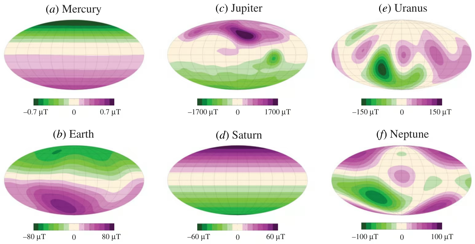
Fig. 4.26 Radial magnetic field at the surfaces of (a) Mercury, (b) Earth, (c) Jupiter, (d) Saturn, (e) Uranus, and (f) Neptune, in Mollweide projections. Earth, Jupiter, and Saturn are predominantly dipolar with the dipole axis approximately aligned with the rotation axis; Uranus and Neptune are clearly multipolar with dipoles tilted by \(\sim 59°\) and \(\sim 47°\) respectively and offset from the planet centre; Mercury’s field is weak and asymmetric, with the dipole offset \(\sim 500\) km northward. Field intensities span four orders of magnitude (note the per-panel colour scales). Reproduced from [Soderlund and Stanley, 2020], Fig. 1.

4.8.2. Dipolar versus multipolar fields

Dynamo regimes depend on the local Rossby number, the ratio of inertial to Coriolis forces (Fig. 4.27).

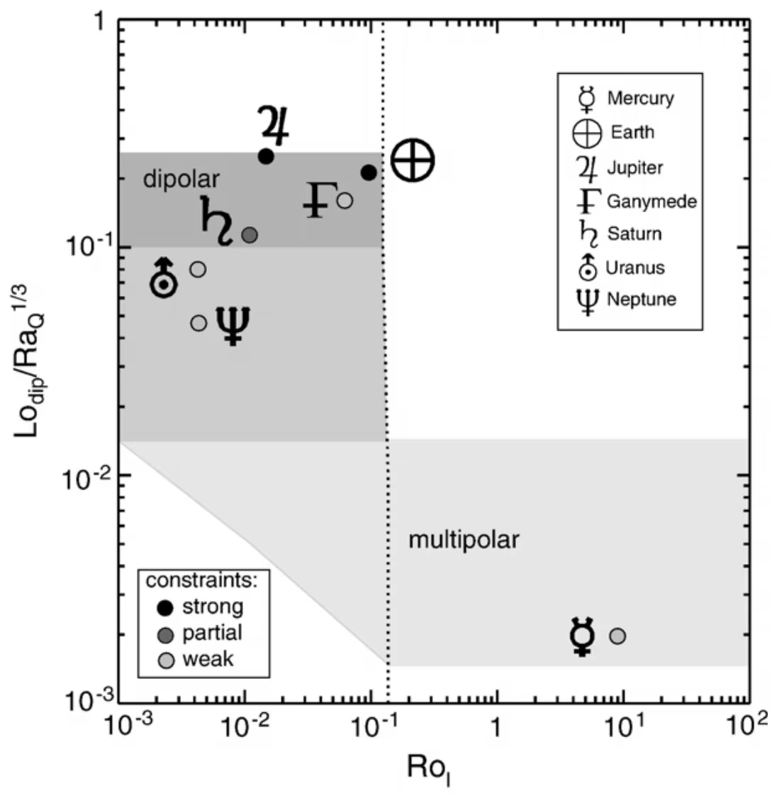
Fig. 4.27 Dimensionless dipole moment (the dipole Lorentz number \(\mathrm{Lo}_{\rm dip}\) scaled by the buoyancy-flux Rayleigh number, \(\mathrm{Lo}_{\rm dip}/\mathrm{Ra}_Q^{1/3}\)) versus local Rossby number \(\mathrm{Ro}_l\). The transition from the strongly dipolar regime (dark shading) to the multipolar regime (light shading) is calibrated against numerical dynamo simulations; the dotted line marks the regime transition at \(\mathrm{Ro}_l \sim 0.1\). The six dynamo-hosting planets and Ganymede are placed at their estimated control-parameter values; the grey circle next to each symbol indicates the strength of the observational constraint. Earth, Jupiter, Saturn, and Ganymede sit in or near the dipolar regime; Uranus and Neptune sit lower, and Mercury falls in the multipolar regime, consistent with their tilted, offset, or weak surface fields. Reproduced from [Olson and Christensen, 2006], Fig. 7.

4.8.3. The dynamo scaling law

The dynamo scaling law relates surface dipole field \(B_\mathrm{dip}\) to convective buoyancy flux \(F_q\) and shell thickness \(D\) [Christensen and Aubert, 2006]:

(4.11)\[ B_\mathrm{dip} \propto \sqrt{\rho_\mathrm{core} \mu_0} \cdot \big( F_q \cdot D \big)^{1/3} \]

where \(\rho_\mathrm{core}\) is fluid density and \(\mu_0\) is free-space permeability. In rapidly rotating cores, convective energy generation sets field strength (Fig. 4.28).

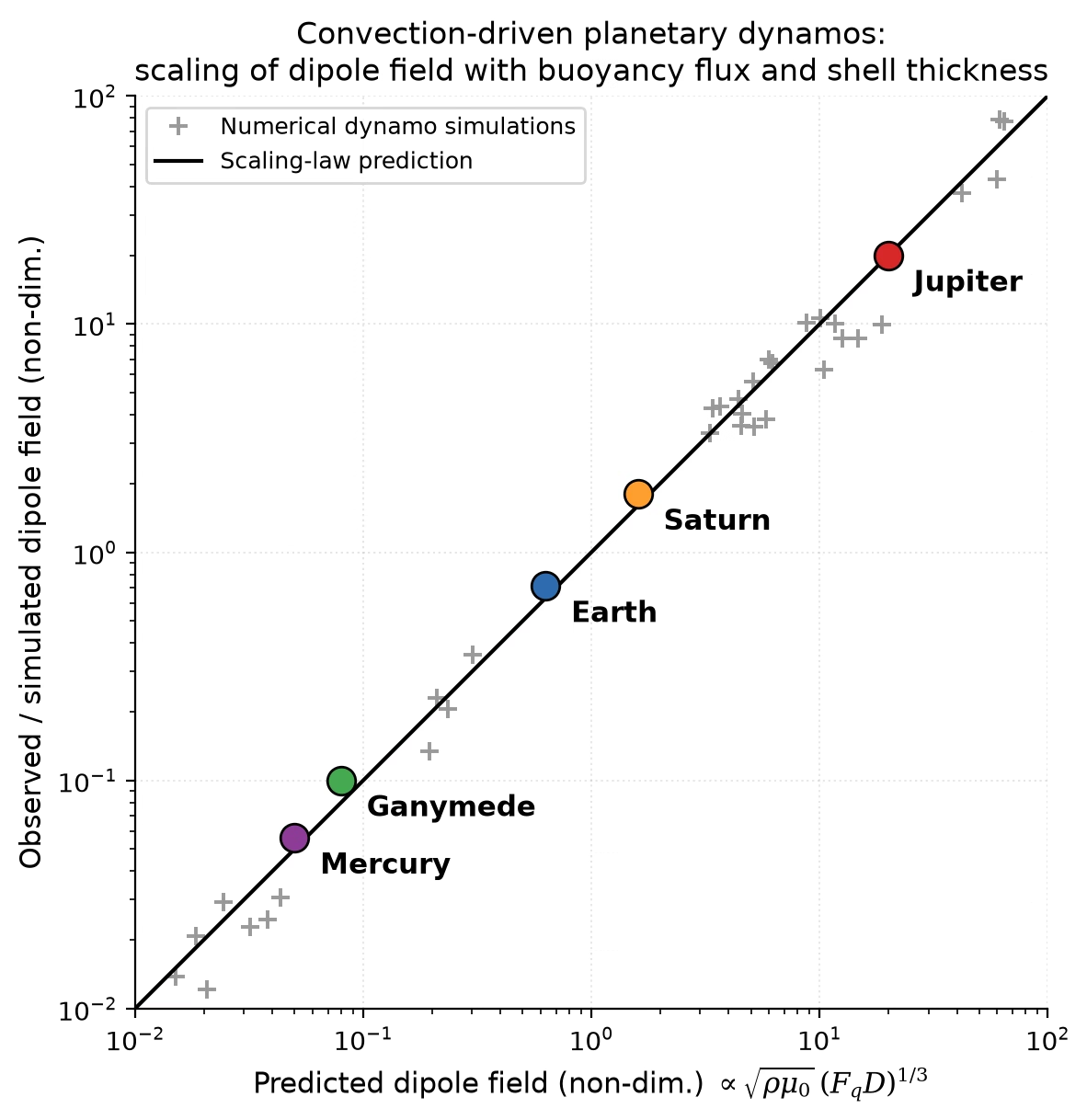
Fig. 4.28 Predicted vs observed magnetic-field strength for convection-driven dynamos, following the scaling law of Eq. (4.11). The horizontal axis is a non-dimensional combination of convective buoyancy flux, shell thickness, and core density; the vertical axis is the measured (observed) or computed (simulated) dipole field. The grey crosses illustrate the published result that numerical dynamo simulations collapse onto a single line over roughly four orders of magnitude; Earth, Jupiter, Saturn, Mercury, and Ganymede (coloured symbols) lie on the same relation within factors of order unity. Venus is omitted because its present-day dynamo is shut off. Illustration after Christensen and Aubert [2006] and Olson and Christensen [2006]. Course-original figure.

4.8.4. Mercury

Mercury possesses a weak but active dynamo: its surface field is only about 1% of Earth’s, and the MESSENGER mission revealed that it is strongly offset northward from the planet’s centre [Anderson et al., 2012]. The liquid part of Mercury’s large core is thought to form only a thin shell, perhaps a few hundred kilometres thick, above a solidifying interior; in the favoured iron-snow scenario, iron crystallises near the top of this shell and the sinking crystals release compositional buoyancy only episodically. The product \(F_q \cdot D\) in Eq. (4.11) is therefore small, and Mercury’s dynamo is intrinsically weak at its source, not merely attenuated on the way to the surface.

4.8.5. Venus

Venus is nearly identical to Earth in size and bulk composition, yet has no detected magnetic field. Slow rotation alone cannot explain this, because dynamo simulations show that even a 243-day rotation period leaves the core rotation-dominated. The leading explanation combines two factors: no solid inner core has nucleated to drive compositional convection, and a stagnant mantle lid (Lecture 9) extracts heat too slowly for thermal convection. In Eq. (4.11), both \(F_q\) and the convecting-shell geometry are suppressed. Venus is thus probably limited not by core composition, but by mantle dynamics controlling core heat loss [de Pater and Lissauer, 2010].

4.8.6. Mars

Mars has no global magnetic field today, but preserves remnant crustal magnetism (patches of crustal magnetisation) in the ancient southern highlands (Fig. 4.29) [Acuña et al., 1999]. The dynamo shut down between \(\sim 4.1\) Ga [Acuña et al., 1999] and \(\sim 3.7\) Ga [Mittelholz et al., 2020], leaving the atmosphere unshielded against solar wind erosion (Lecture 10).

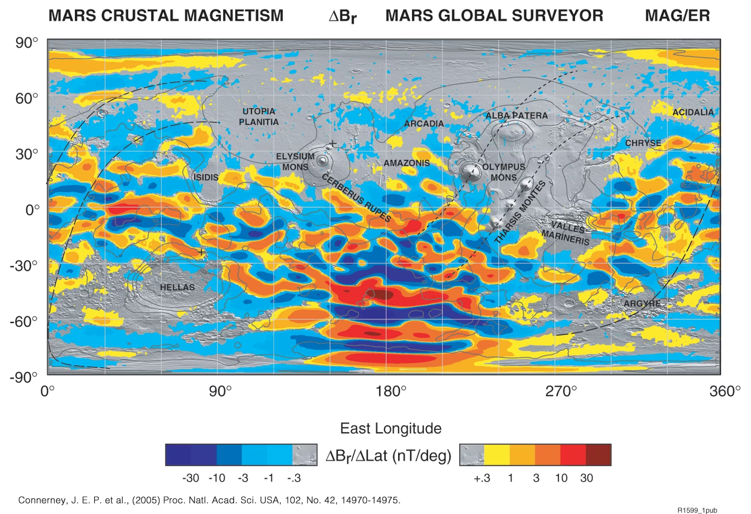
Fig. 4.29 Global map of the radial component \(\Delta B_r\) of Mars’s crustal magnetic field, compiled from Mars Global Surveyor (MGS) magnetometer / electron-reflectometer (MAG/ER) data at \(\sim 400\) km mapping-orbit altitude. Red and blue regions indicate strong crustal magnetisation in opposite polarities, concentrated in the ancient southern highlands. The younger northern lowlands and the large impact basins (Hellas, Argyre, Isidis) show little to no magnetisation, indicating the dynamo had ceased before these features formed [Connerney et al., 2005]. The original detection of Mars’s crustal field is reported in Acuña et al. [1999]. Credit: NASA/Goddard Space Flight Center, public domain.

4.8.7. Jupiter

Convection in metallic hydrogen (an electrical conductor at pressures above \(\sim\)100 GPa) generates Jupiter’s asymmetric magnetic field (Fig. 4.30) [Connerney et al., 2022].

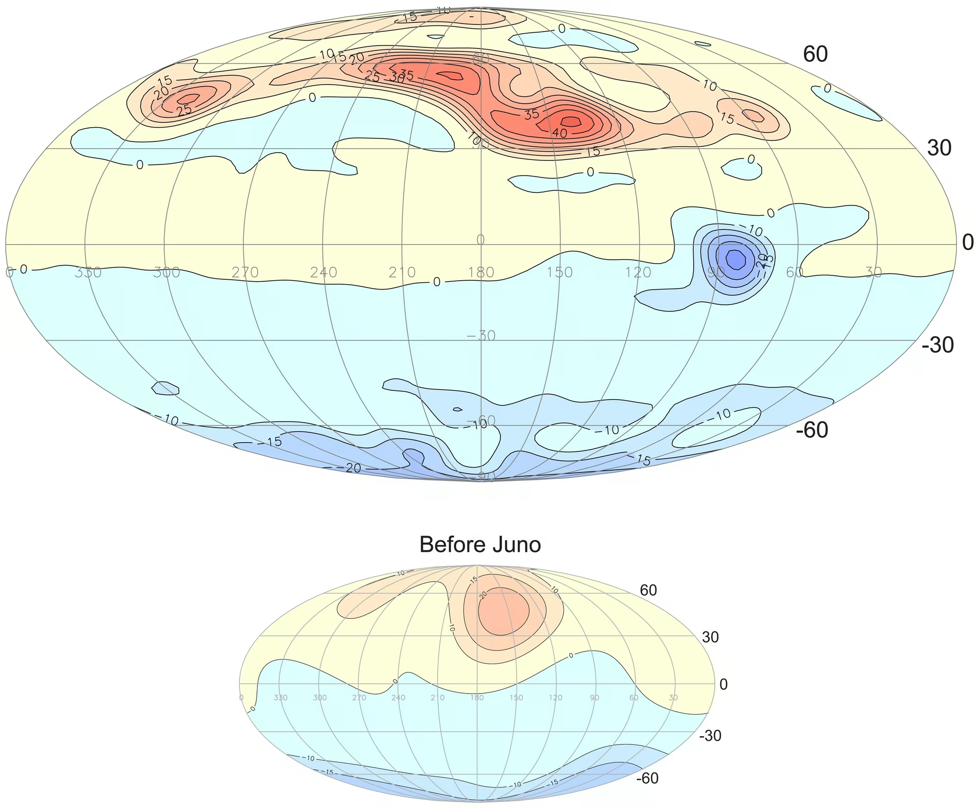
Fig. 4.30 Radial component of Jupiter’s surface magnetic field from a field model built from the orbits of Juno’s prime mission (top), compared with the pre-Juno picture assembled from earlier missions (Pioneer 10 and 11, Voyager 1 and 2, Ulysses, and Galileo; bottom) [Connerney et al., 2022]. Field lines emerge from the planet in the yellow and red regions and enter it in the blue regions. Unlike Earth’s field, which is dominated by an axial dipole at the surface, Jupiter’s surface field shows pronounced non-dipolar structure, most strikingly the intense localised patch of inward flux near the equator (the “Great Blue Spot”). This morphology constrains the depth at which the metallic-hydrogen dynamo operates. Credit: NASA/JPL-Caltech/SwRI/J.E.P. Connerney (PIA25040), public domain.

4.8.8. Ganymede

Ganymede (\(R = 2634\) km) is the only moon with an intrinsic dynamo, generated in a liquid iron shell around a crystallising inner core [de Pater and Lissauer, 2010]. Because its core is small (\(R_\mathrm{core} \sim 700\) km) and deep, the surface retains only \((R_\mathrm{core}/R_\mathrm{body})^3 \approx 2\%\) of the dynamo-region field. Yet Ganymede’s surface field (\(\sim 0.7\) \(\mu\)T) exceeds Mercury’s (\(\sim 0.3\) \(\mu\)T), which points to a larger \(F_q \cdot D\) product in Eq. (4.11) sustained by steadier compositional buoyancy than Mercury’s episodic iron snow.

Fig. 4.31 collects the dynamo state of the terrestrial bodies and Ganymede; the lunar paleofield and the inner-core age return under Recent advances.

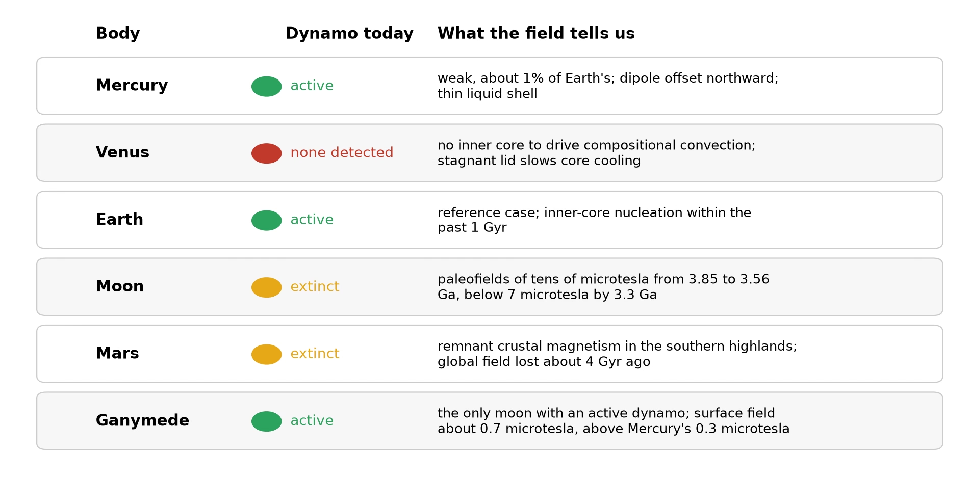
Fig. 4.31 Dynamo status of the terrestrial bodies and Ganymede, the only moon with an active dynamo: Mercury (weak active dynamo, surface field about 1% of Earth’s, offset northward), Venus (no detected field, no inner core and a stagnant lid), Earth (active, inner-core nucleation within the past 1 Gyr), the Moon (extinct, with paleofields of tens of microtesla from 3.85 to 3.56 Ga), Mars (extinct, remnant crustal magnetism, global field lost about 4 Gyr ago) and Ganymede (active, surface field about 0.7 \(\mu\)T against Mercury’s 0.3 \(\mu\)T). Course-original figure.

4.9. Magnetosphere-solar wind interaction

A planetary magnetic field does not exist in isolation: it interacts dynamically with the solar wind, the continuous stream of charged particles (mostly protons and electrons) flowing outward from the Sun at speeds of 300–800 km s\(^{-1}\), carrying an embedded magnetic field (the interplanetary magnetic field, or IMF) [Kivelson and Russell, 1995].

4.9.1. Magnetopause and magnetosphere structure

The magnetopause is the boundary where solar wind ram pressure balances planetary magnetic pressure:

(4.12)\[ \frac{1}{2} \rho_{\mathrm{sw}} v_{\mathrm{sw}}^2 = \frac{B_{\mathrm{mp}}^2}{2\mu_0} \]

where \(\rho_{\mathrm{sw}}\) and \(v_{\mathrm{sw}}\) are solar wind density and velocity, and \(B_{\mathrm{mp}}\) is magnetic field strength. For a dipole field (\(B \propto r^{-3}\)), this sets the standoff distance:

(4.13)\[ r_{\mathrm{mp}} \approx 10 \, R_\oplus \]

for Earth under typical solar wind conditions (Fig. 4.32).

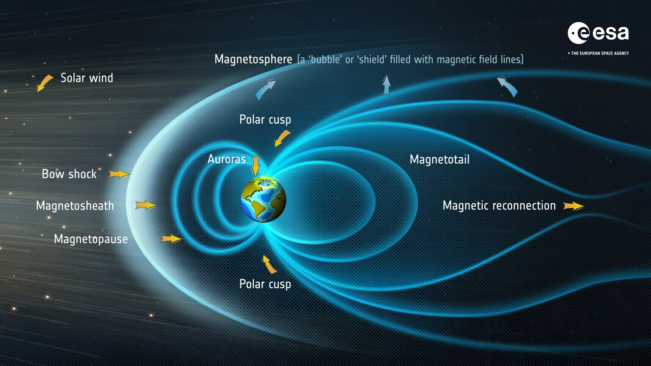
Fig. 4.32 Anatomy of Earth’s magnetosphere. The solar wind (orange arrows, arriving from the left) is slowed and deflected at the bow shock, and the shocked plasma flows around the planet through the turbulent magnetosheath. The magnetopause is the surface where the solar wind ram pressure is balanced by the magnetic pressure of Earth’s field (Eq. (4.12)); under typical conditions it lies at the standoff distance \(r_{\mathrm{mp}} \approx 10\,R_\oplus\). Inside it, the dayside field is compressed, while the nightside field is stretched into the long magnetotail. Credit: ESA, CC BY-SA 3.0 IGO.

4.9.2. Auroral processes

An aurora is light emitted when charged particles channelled along magnetic field lines excite atmospheric gas (Fig. 4.33, Fig. 4.34) [Kivelson and Russell, 1995].

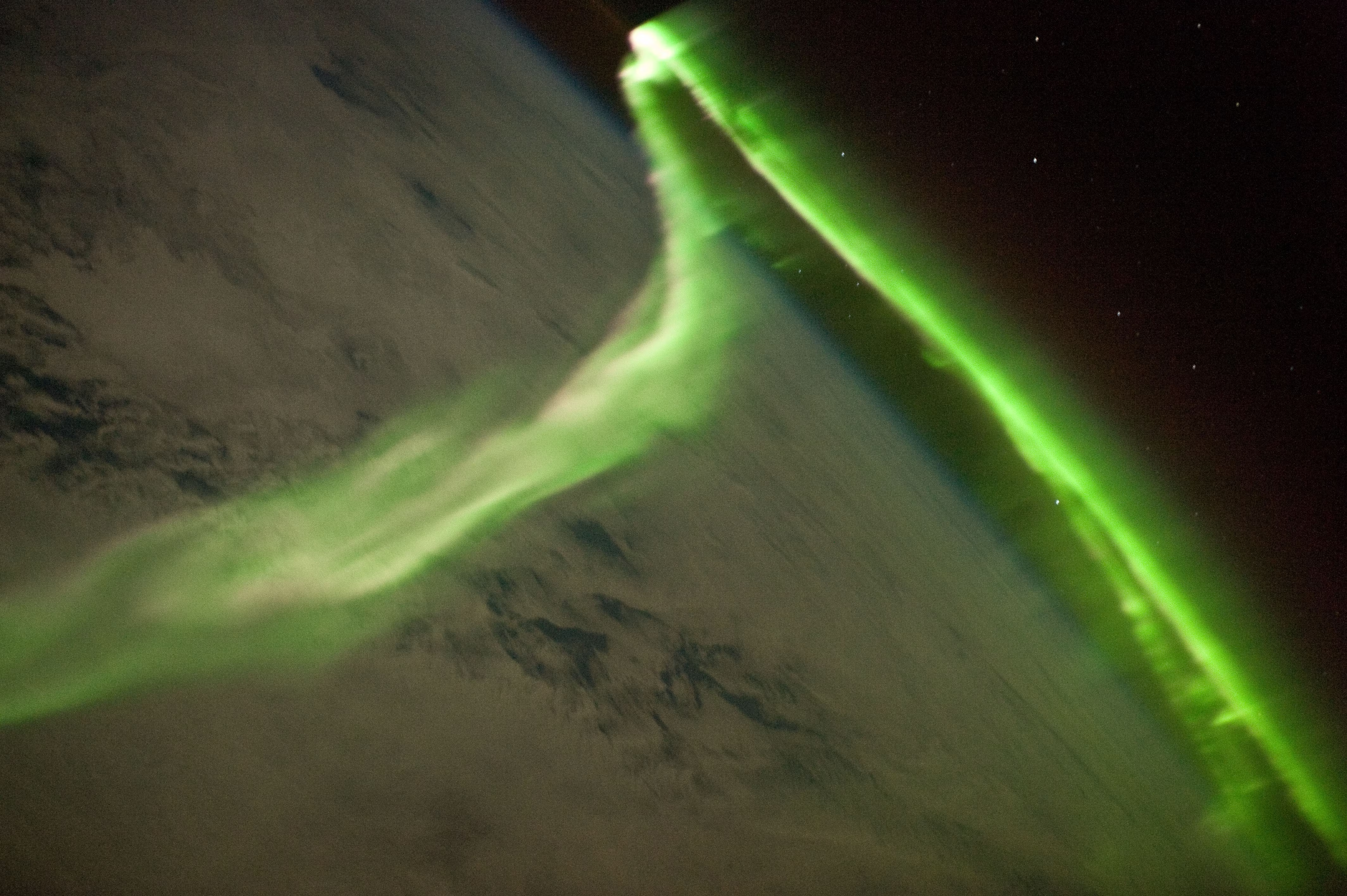
Fig. 4.33 The aurora australis (southern lights) photographed from the International Space Station. Charged particles from the solar wind, channelled along Earth’s magnetic field lines into the polar regions, excite atmospheric oxygen and nitrogen to produce the characteristic green and red glow. Credit: NASA/ISS Crew Earth Observations, public domain.

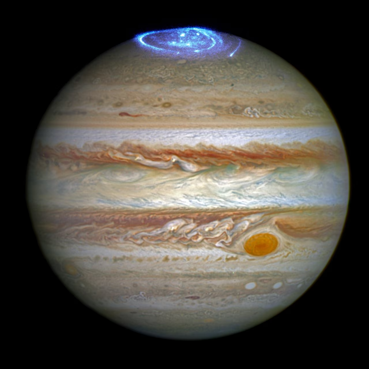
Fig. 4.34 Ultraviolet aurora at Jupiter’s north pole, imaged by the Hubble Space Telescope. The bright auroral oval is powered by Jupiter’s rapid rotation, by particles from the Io plasma torus, and by interactions with the solar wind, making it the most luminous aurora in the solar system; Jovian aurorae are largely persistent rather than driven by solar wind variability as on Earth. The composite shows the UV aurora overlaid on an optical Hubble image of the planet. Credit: NASA, ESA, J. Nichols (University of Leicester).

4.9.3. Van Allen radiation belts

The Van Allen radiation belts are two toroidal regions where Earth’s magnetosphere traps energetic charged particles (Fig. 4.35) [de Pater and Lissauer, 2010]. These trapped particles pose hazards to spacecraft and astronauts, showing that magnetic fields shield the surface while trapping energetic radiation.

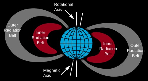
Fig. 4.35 Cross-section of Earth’s Van Allen radiation belts. The inner belt of energetic protons (10–100 MeV) is centred at \(\sim 1.5\,R_\oplus\) and is largely stable; the outer belt of energetic electrons (0.1–10 MeV) is centred at \(\sim 4\)–\(5\,R_\oplus\) and is highly variable, expanding and contracting in response to geomagnetic storms. Both populations are confined to closed magnetic field lines that thread the inner magnetosphere. Credit: Booyabazooka / NASA, public domain (Wikimedia Commons).

4.10. Recent advances

NASA’s Juno mission has produced the most detailed map of Jupiter’s magnetic field to date [Connerney et al., 2022]. The data reveal a surprisingly complex field morphology: in the northern hemisphere, the field shows strong non-dipolar features, including a localised patch of reversed polarity (the “Great Blue Spot”) that may reflect the dynamics of a deep-seated dynamo operating in the metallic hydrogen layer (Lecture 8). These measurements provide direct constraints on the depth and nature of convection driving Jupiter’s dynamo.

4.10.1. InSight: no present-day Mars dynamo

NASA’s InSight lander detected no global dynamo field on Mars [Johnson et al., 2020]. Seismic data indicate a fully liquid core (Fig. 4.36) [Stähler et al., 2021]. Without compositional buoyancy from inner-core growth, thermal convection ceased once initial heat was lost (Lecture 10).

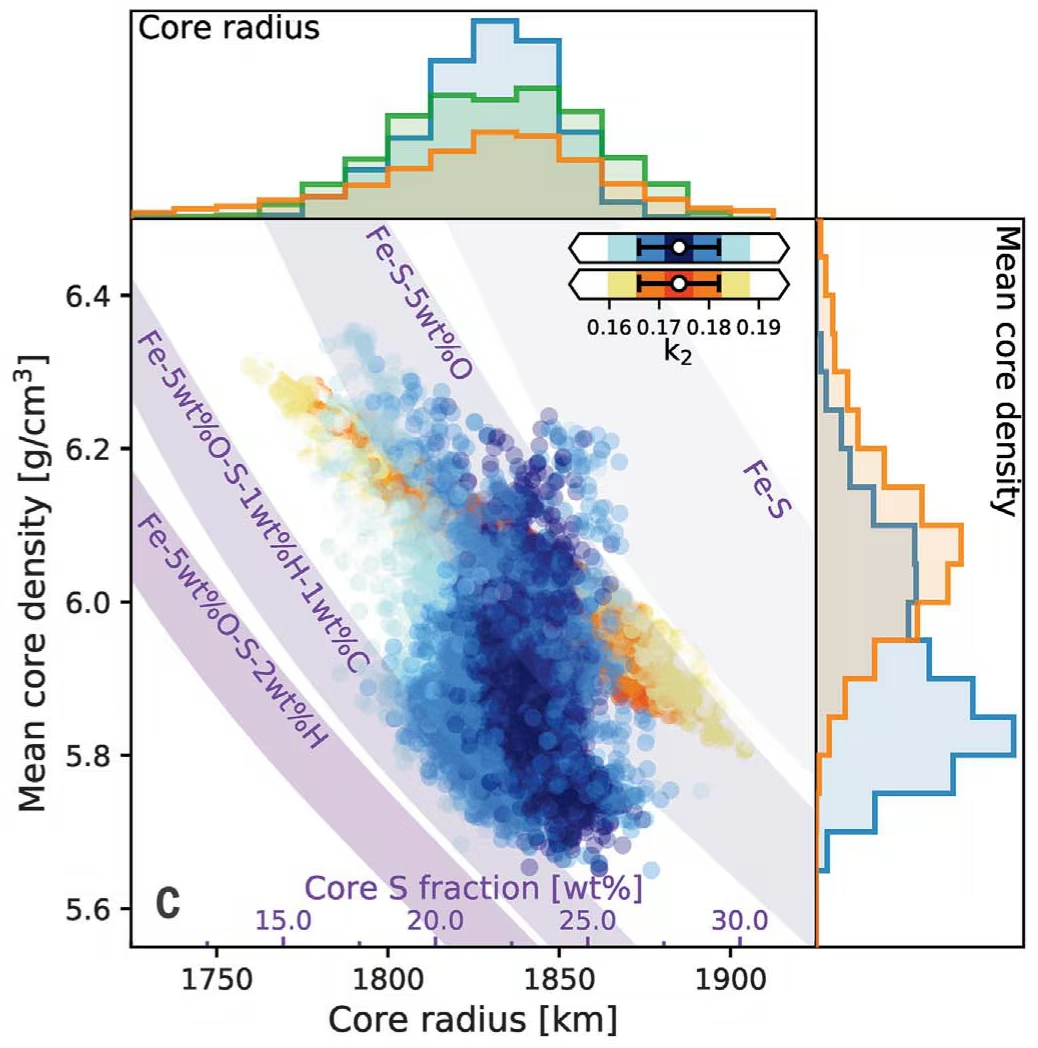
Fig. 4.36 Sampled core properties of Mars from InSight. The central panel shows mean core density versus core radius for models from the geophysical (blue shades) and geodynamical (warm shades, yellow to red) inversions, with each point colour-coded by how well the model fits the observed degree-2 tidal Love number \(k_2\) (inset), a dimensionless measure of how much a body’s mass redistributes in response to tidal forcing. Marginal histograms are shown at the top and right; the purely seismic inversion (green histogram) constrains only the core radius. All three methods converge on a core radius near 1830 km, and the implied mean core density of \(\sim 6\) g cm\(^{-3}\) is too low for pure iron: the purple bands, which trace the core sulfur content of Fe alloys with light elements (S, O, H, C), require several wt% of light elements. Reproduced from Stähler et al. [2021], Fig. 2C.

4.10.2. The lunar dynamo paradox

Paleomagnetic measurements of Apollo samples have established that the Moon itself once hosted a core dynamo. The remanent magnetisation of lunar rocks returned by Apollo 15, 16, and 17 implies paleofield strengths of tens of microtesla in the high-field epoch from \(\sim 3.85\) to \(\sim 3.56\) Ga (mean \(\sim 77\,\mu\)T), dropping below \(\sim 7\,\mu\)T by \(\sim 3.3\) Ga [Weiss and Tikoo, 2014]. A microtesla-scale field at a body with only \(\sim 400\) km liquid core radius is difficult to generate by purely thermal convection; proposed mechanisms include differential rotation of the core driven by tidal or impact-induced torques, and compositional buoyancy from core crystallisation similar to the scenarios proposed for Mercury and Ganymede (Fig. 4.28).

Fig. 4.37 places these numbers on an age axis.

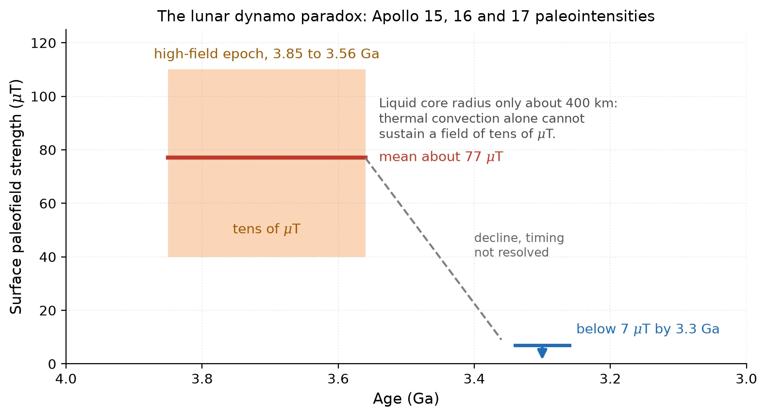
Fig. 4.37 The lunar dynamo paradox: surface paleofield strength recorded by the Apollo 15, 16 and 17 samples against age. The high-field epoch from about 3.85 to 3.56 Ga has a mean of about 77 \(\mu\)T (tens of microtesla, shaded), and the field had dropped below 7 \(\mu\)T by about 3.3 Ga [Weiss and Tikoo, 2014]. A field of tens of microtesla from a liquid core of only about 400 km radius is difficult to generate by thermal convection alone. Course-original figure.

4.10.3. The Earth inner-core age debate

Earth’s inner core grows by the freezing of liquid iron at its surface, and the time when this inner-core nucleation started is not settled: published estimates range from about 0.55 to 2 Gyr ago. The debate has three parts: the thermal conductivity of the core, the reading of the paleomagnetic record, and the power source of the geodynamo before the inner core existed.

The first part is the thermal conductivity of iron at core conditions, which sets how much heat conducts down the core adiabat without driving convection. First-principles calculations and resistivity measurements in the diamond-anvil cell give a conductivity two to three times larger than the traditional value, so the core cools fast and the inner core is young, less than about 1 Gyr [Labrosse, 2015, Ohta et al., 2016]. Direct measurements of the thermal conductivity of solid iron give 18 to 44 W m\(^{-1}\) K\(^{-1}\), near the low end of earlier estimates, which allows an inner core as old as the dynamo itself [Konôpková et al., 2016].

The second part is the paleomagnetic record. Nucleation adds compositional convection and latent heat as buoyancy sources, so the field strength is expected to rise when it starts. A compilation of Precambrian paleointensities shows a rise in average field strength and variability between 1.0 and 1.5 Ga, interpreted as a Mesoproterozoic nucleation that favours a modest conductivity [Biggin et al., 2015]. Single-crystal paleointensities from Ediacaran rocks instead record an ultralow field at about 565 Ma, followed by a five-fold renewal by about 532 Ma, which places nucleation near 0.55 Ga [Bono et al., 2019, Zhou et al., 2022]. A high conductivity favours the younger age, in which case the 1.0 to 1.5 Ga rise has another cause [Ohta et al., 2016].

The third part is the power source of the geodynamo (the mechanism generating Earth’s magnetic field) before nucleation, the new core paradox [Olson, 2013]. Single silicate crystals record a geodynamo at 3.4 to 3.45 Ga with 50 to 70 percent of the present field strength [Tarduno et al., 2010]. With a high conductivity, thermal convection and radiogenic heating alone may not have been able to sustain the geodynamo through those early epochs, because most of the core heat flow then conducts along the adiabat instead of convecting [O'Rourke and Stevenson, 2016]. Proposed resolutions are a lower conductivity, a much hotter early core with a high core-mantle heat flow, or an extra compositional buoyancy source before nucleation, such as the precipitation of magnesium-bearing minerals from the cooling core [O'Rourke and Stevenson, 2016].

Fig. 4.38 places the estimates on a timeline.

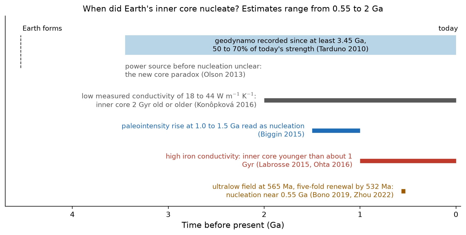
Fig. 4.38 The inner-core age debate on a timeline. A geodynamo is recorded from at least 3.45 Ga [Tarduno et al., 2010], and how it was powered before the inner core existed is the new core paradox [Olson, 2013]. Nucleation estimates run from 0.55 to 2 Ga: a high thermal conductivity of iron gives an inner core younger than about 1 Gyr [Labrosse, 2015, Ohta et al., 2016], a low measured conductivity allows an inner core 2 Gyr old or older [Konôpková et al., 2016], a paleointensity rise at 1.0 to 1.5 Ga is read as nucleation [Biggin et al., 2015], and an ultralow field at 565 Ma followed by renewal places it near 0.55 Ga [Bono et al., 2019, Zhou et al., 2022]. Course-original figure.

4.10.4. BepiColombo, JUICE, and Europa Clipper

The ESA/JAXA BepiColombo mission (orbital insertion late \(2026\)) provides measurements of Mercury’s weak dipolar magnetic field. Operating two orbiters simultaneously will correlate in-situ magnetospheric measurements with surface and interior constraints [Benkhoff et al., 2021].

ESA’s JUICE mission will investigate Ganymede, the only moon in the solar system known to generate its own dynamo. How a body as small as Ganymede (\(R = 2634\) km) maintains an active dynamo constrains the thermal state and composition of its iron core.

NASA’s Europa Clipper (launched 2024, arriving at Jupiter in 2030) carries a magnetometer to measure the induced magnetic signature of Europa’s subsurface ocean. Measuring this induced response to Jupiter’s ambient field constrains ocean salinity, ocean thickness, and core thermal state (Lecture 8). This provides magnetic-field remote sensing of Europa’s interior, with habitability implications explored in Lecture 14.

4.11. Looking ahead to Lecture 5

This lecture ended with a planet that has a core, a mantle, a magnetic field, and a freshly outgassed secondary atmosphere. Lecture 5 picks up that atmosphere and asks what it looks like: how primary, secondary, and tertiary atmospheres differ, how pressure and temperature vary with height under hydrostatic equilibrium, how the greenhouse effect sets the surface temperature, and how atmospheres are lost to space. The magnetic shielding story from this lecture returns there as one control on escape, alongside the thermal escape processes that magnetic fields cannot stop.

4.12. References

[Acuna1999] (1,2,3)

Acuña, Mario H., Connerney, John E. P., Ness, Norman F., Lin, Robert P., Mitchell, David, Carlson, Charles W., McFadden, James, Anderson, K. A., Rème, Henri, Mazelle, Christian, Vignes, Danièle, Wasilewski, Peter, and Cloutier, Paul. 1999. “Global distribution of crustal magnetization discovered by the Mars Global Surveyor MAG/ER experiment.” Science, 284(5415):790–793. doi:10.1126/science.284.5415.790, https://ui.adsabs.harvard.edu/abs/1999Sci...284..790A/abstract.

[Alexander2019b]

Alexander, Conel M. O'D. 2019. “Quantitative models for the elemental and isotopic fractionations in chondrites: The carbonaceous chondrites.” Geochimica et Cosmochimica Acta, 254:277–309. doi:10.1016/j.gca.2019.02.008, https://ui.adsabs.harvard.edu/abs/2019GeCoA.254..277A/abstract.

[Alexander2019a]

Alexander, Conel M. O'D. 2019. “Quantitative models for the elemental and isotopic fractionations in the chondrites: The non-carbonaceous chondrites.” Geochimica et Cosmochimica Acta, 254:246–276. doi:10.1016/j.gca.2019.01.026, https://ui.adsabs.harvard.edu/abs/2019GeCoA.254..246A/abstract.

[Anderson2012]

Anderson, Brian J., Johnson, Catherine L., Korth, Haje, Winslow, Reka M., Borovsky, Joseph E., Purucker, Michael E., Slavin, James A., Solomon, Sean C., Zuber, Maria T., and McNutt, Jr., Ralph L. 2012. “Low-degree structure in Mercury's planetary magnetic field.” Journal of Geophysical Research: Planets, 117:E00L12. doi:10.1029/2012JE004159, https://ui.adsabs.harvard.edu/abs/2012JGRE..117.0L12A/abstract.

[AndrewsHanna2008]

Andrews-Hanna, Jeffrey C., Zuber, Maria T., and Banerdt, W. Bruce. 2008. “The Borealis basin and the origin of the martian crustal dichotomy.” Nature, 453(7199):1212–1215. doi:10.1038/nature07011, https://ui.adsabs.harvard.edu/abs/2008Natur.453.1212A/abstract.

[Benkhoff2021]

Benkhoff, Johannes, Murakami, Go, Baumjohann, Wolfgang, Besse, Sébastien, Bunce, Emma, Casale, Marina, Cremosese, Gabriele, Glassmeier, Karl-Heinz, Hayakawa, Hajime, Heyner, Daniel, Hiesinger, Harald, Huovelin, Juhani, Hussmann, Hauke, Iafolla, Valerio, Iess, Luciano, Kasaba, Yasumasa, Kobayashi, Masanori, Milillo, Anna, Mitrofanov, Igor G., Montagnon, Eric, Novara, Maria, Orsini, Stefano, Quemerais, Eric, Reininghaus, Ulrich, Saito, Yoshifumi, Santoli, Francesco, Stramaccioni, Daniele, Sutherland, Olivier, Thomas, Nicolas, Yoshikawa, Ichiro, and Zender, Joe. 2021. “BepiColombo: Mission overview and science goals.” Space Science Reviews, 217(8):90. doi:10.1007/s11214-021-00861-4, https://ui.adsabs.harvard.edu/abs/2021SSRv..217...90B/abstract.

[Benz2007]

Benz, W., Anic, A., Horner, J., and Whitby, J. A. 2007. “The origin of Mercury.” Space Science Reviews, 132(2–4):189–202. doi:10.1007/s11214-007-9284-1, https://ui.adsabs.harvard.edu/abs/2007SSRv..132..189B/abstract.

[Benz1988]

Benz, W., Slattery, W. L., and Cameron, A. G. W. 1988. “Collisional stripping of Mercury's mantle.” Icarus, 74(3):516–528. doi:10.1016/0019-1035(88)90118-2, https://ui.adsabs.harvard.edu/abs/1988Icar...74..516B/abstract.

[Biggin2015] (1,2)

Biggin, A. J., Piispa, E. J., Pesonen, L. J., Holme, R., Paterson, G. A., Veikkolainen, T., and Tauxe, L. 2015. “Palaeomagnetic field intensity variations suggest Mesoproterozoic inner-core nucleation.” Nature, 526(7572):245–248. doi:10.1038/nature15523.

[Bono2019] (1,2)

Bono, Richard K., Tarduno, John A., Nimmo, Francis, and Cottrell, Rory D. 2019. “Young inner core inferred from Ediacaran ultra-low geomagnetic field intensity.” Nature Geoscience, 12(2):143–147. doi:10.1038/s41561-018-0288-0.

[Chau2018] (1,2,3)

Chau, Alice, Reinhardt, Christian, Helled, Ravit, and Stadel, Joachim. 2018. “Forming Mercury by giant impacts.” The Astrophysical Journal, 865(1):35. doi:10.3847/1538-4357/aad8b0, arXiv:1808.07473, https://ui.adsabs.harvard.edu/abs/2018ApJ...865...35C/abstract.

[ChristensenAubert2006] (1,2)

Christensen, U. R. and Aubert, J. 2006. “Scaling properties of convection-driven dynamos in rotating spherical shells and application to planetary magnetic fields.” Geophysical Journal International, 166(1):97–114. doi:10.1111/j.1365-246X.2006.03009.x, https://ui.adsabs.harvard.edu/abs/2006GeoJI.166...97C/abstract.

[Connerney2005]

Connerney, J. E. P., Acuña, M. H., Ness, N. F., Kletetschka, G., Mitchell, D. L., Lin, R. P., and Reme, H. 2005. “Tectonic implications of Mars crustal magnetism.” Proceedings of the National Academy of Sciences, 102(42):14970–14975. doi:10.1073/pnas.0507469102, https://ui.adsabs.harvard.edu/abs/2005PNAS..10214970C/abstract.

[Connerney2022] (1,2,3)

Connerney, J. E. P., Timmins, S., Oliversen, R. J., Espley, J. R., Joergensen, J. L., Kotsiaros, S., Joergensen, P. S., Merayo, J. M. G., Herceg, M., Bloxham, J., Moore, K. M., Bolton, S. J., and Levin, S. M. 2022. “A new model of Jupiter's magnetic field at the completion of Juno's prime mission.” Journal of Geophysical Research: Planets, 127(2):e2021JE007055. doi:10.1029/2021JE007055, https://ui.adsabs.harvard.edu/abs/2022JGRE..12707055C/abstract.

[dePaterLissauer2010] (1,2,3)

de Pater, Imke and Lissauer, Jack J. 2010. Planetary Sciences. Cambridge University Press, Cambridge, 2nd edition. doi:10.1017/cbo9780511780561.

[Dziewonski1981] (1,2)

Dziewonski, Adam M. and Anderson, Don L. 1981. “Preliminary reference Earth model.” Physics of the Earth and Planetary Interiors, 25(4):297–356. doi:10.1016/0031-9201(81)90046-7, https://ui.adsabs.harvard.edu/abs/1981PEPI...25..297D/abstract.

[ElkinsTanton2012] (1,2,3,4)

Elkins-Tanton, Linda T. 2012. “Magma oceans in the inner solar system.” Annual Review of Earth and Planetary Sciences, 40:113–139. doi:10.1146/annurev-earth-042711-105503, https://ui.adsabs.harvard.edu/abs/2012AREPS..40..113E/abstract.

[Fischer2015] (1,2,3)

Fischer, Rebecca A., Nakajima, Yoichi, Campbell, Andrew J., Frost, Daniel J., Harries, Dennis, Langenhorst, Falko, Miyajima, Nobuyoshi, Pollok, Kilian, and Rubie, David C. 2015. “High pressure metal–silicate partitioning of Ni, Co, V, Cr, Si, and O.” Geochimica et Cosmochimica Acta, 167:177–194. doi:10.1016/j.gca.2015.06.026.

[GendaAbe2003]

Genda, H. and Abe, Y. 2003. “Survival of a proto-atmosphere through the stage of giant impacts: the mechanical aspects.” Icarus, 164(1):149–162. doi:10.1016/S0019-1035(03)00101-5, https://ui.adsabs.harvard.edu/abs/2003Icar..164..149G/abstract.

[GendaAbe2005]

Genda, H. and Abe, Y. 2005. “Enhanced atmospheric loss on protoplanets at the giant impact phase in the presence of oceans.” Nature, 433(7028):842–844. doi:10.1038/nature03360, https://ui.adsabs.harvard.edu/abs/2005Natur.433..842G/abstract.

[Gradstein2020]

Gradstein, Felix M., Ogg, James G., Schmitz, Mark D., and Ogg, Gabi M., editors. 2020. Geologic Time Scale 2020. Elsevier. doi:10.1016/C2020-1-02369-3, https://www.sciencedirect.com/book/9780128243602/geologic-time-scale-2020.

[Grewal2021]

Grewal, Damanveer S., Dasgupta, Rajdeep, and Marty, Bernard. 2021. “A very early origin of isotopically distinct nitrogen in inner Solar System protoplanets.” Nature Astronomy, 5:356–364. doi:10.1038/s41550-020-01283-y, https://ui.adsabs.harvard.edu/abs/2021NatAs...5..356G/abstract.

[Grewal2024] (1,2)

Grewal, Damanveer S., Nie, Nicole X., Zhang, Bidong, Izidoro, Andre, and Asimow, Paul D. 2024. “Accretion of the earliest inner Solar System planetesimals beyond the water snowline.” Nature Astronomy, 8:290–297. doi:10.1038/s41550-023-02172-w, https://doi.org/10.1038/s41550-023-02172-w.

[Hin2017]

Hin, Remco C., Coath, Christopher D., Carter, Philip J., Nimmo, Francis, Lai, Yi-Jen, Pogge von Strandmann, Philip A. E., Willbold, Matthias, Leinhardt, Zoë M., Walter, Michael J., and Elliott, Tim. 2017. “Magnesium isotope evidence that accretional vapour loss shapes planetary compositions.” Nature, 549:511–515. doi:10.1038/nature23899, https://doi.org/10.1038/nature23899.

[Hirschmann2012] (1,2)

Hirschmann, Marc M. 2012. “Magma ocean influence on early atmosphere mass and composition.” Earth and Planetary Science Letters, 341–344:48–57. doi:10.1016/j.epsl.2012.06.015, https://ui.adsabs.harvard.edu/abs/2012E&PSL.341...48H/abstract.

[Johansen2021]

Johansen, Anders, Ronnet, Thomas, Bizzarro, Martin, Schiller, Martin, Lambrechts, Michiel, Nordlund, Åke, and Lammer, Helmut. 2021. “A pebble accretion model for the formation of the terrestrial planets in the Solar System.” Science Advances, 7:eabc0444. doi:10.1126/sciadv.abc0444, https://doi.org/10.1126/sciadv.abc0444.

[Johnson2020]

Johnson, Catherine L., Mittelholz, Anna, Langlais, Benoît, Russell, Christopher T., Ansan, Veronique, Banfield, Don, Christensen, Peter R., Constable, Catherine, Déhant, Véronique, Fillingim, Matthew, Forget, François, Haviland, Heidi F., Golombek, Matthew, Joy, Steven, Lognonné, Philippe, Liu, Xinping, Menvielle, Michel, Oliveira, Joana S., Pike, W. Thomas, Smrekar, Suzanne, Spiga, Aymeric, and Spohn, Tilman. 2020. “Crustal and time-varying magnetic fields at the InSight landing site on Mars.” Nature Geoscience, 13:199–204. doi:10.1038/s41561-020-0537-x, https://ui.adsabs.harvard.edu/abs/2020NatGe..13..199J/abstract.

[Kegerreis2022] (1,2)

Kegerreis, J. A., Ruiz-Bonilla, S., Eke, V. R., Massey, R. J., Sandnes, T. D., and Teodoro, L. F. A. 2022. “Immediate origin of the Moon as a post-impact satellite.” The Astrophysical Journal Letters, 937(2):L40. doi:10.3847/2041-8213/ac8d96, arXiv:2210.01814.

[Kivelson1995] (1,2)

Kivelson, Margaret G. and Russell, Christopher T. 1995. Introduction to Space Physics. Cambridge University Press, Cambridge. doi:10.1017/9781139878296.

[Kleine2009]

Kleine, Thorsten, Touboul, Mathieu, Bourdon, Bernard, Nimmo, Francis, Mezger, Klaus, Palme, Herbert, Jacobsen, Stein B., Yin, Qing-Zhu, and Halliday, Alex N. 2009. “Hf–W chronology of the accretion and early evolution of asteroids and terrestrial planets.” Geochimica et Cosmochimica Acta, 73(17):5150–5188. doi:10.1016/j.gca.2008.11.047, https://ui.adsabs.harvard.edu/abs/2009GeCoA..73.5150K/abstract.

[KleineWalker2017] (1,2,3,4,5)

Kleine, Thorsten and Walker, Richard J. 2017. “Tungsten isotopes in planets.” Annual Review of Earth and Planetary Sciences, 45:389–417. doi:10.1146/annurev-earth-063016-020037.

[Konopkova2016] (1,2)

Konôpková, Zuzana, McWilliams, R. Stewart, Gómez-Pérez, Natalia, and Goncharov, Alexander F. 2016. “Direct measurement of thermal conductivity in solid iron at planetary core conditions.” Nature, 534(7605):99–101. doi:10.1038/nature18009.

[Krijt2023] (1,2)

Krijt, Sebastiaan, Kama, Mihkel, McClure, Melissa, Teske, Johanna, Bergin, Edwin A., Shorttle, Oliver, Walsh, Kevin J., and Raymond, Sean N. 2023. “Chemical habitability: supply and retention of life's essential elements during planet formation.” In Inutsuka, Shu-ichiro, Aikawa, Yuri, Muto, Takayuki, Tomida, Kengo, and Tamura, Motohide, editors, Protostars and Planets VII. ASP Conference Series. doi:10.48550/arXiv.2203.10056, arXiv:2203.10056, https://ui.adsabs.harvard.edu/abs/2023ASPC..534.1031K/abstract.

[Kruijer2017Mars] (1,2,3)

Kruijer, Thomas S., Kleine, Thorsten, Borg, Lars E., Brennecka, Gregory A., Irving, Anthony J., Bischoff, Addi, and Agee, Carl B. 2017. “The early differentiation of Mars inferred from Hf-W chronometry.” Earth and Planetary Science Letters, 474:345–354. doi:10.1016/j.epsl.2017.06.047, https://ui.adsabs.harvard.edu/abs/2017E\%26PSL.474..345K/abstract.

[Labrosse2015] (1,2)

Labrosse, Stéphane. 2015. “Thermal evolution of the core with a high thermal conductivity.” Physics of the Earth and Planetary Interiors, 247:36–55. doi:10.1016/j.pepi.2015.02.002, https://ui.adsabs.harvard.edu/abs/2015PEPI..247...36L/abstract.

[Labrosse2007]

Labrosse, Stéphane, Hernlund, John W., and Coltice, Nicolas. 2007. “A crystallizing dense magma ocean at the base of the Earth's mantle.” Nature, 450(7171):866–869. doi:10.1038/nature06355, https://ui.adsabs.harvard.edu/abs/2007Natur.450..866L/abstract.

[Lichtenberg2021]

Lichtenberg, Tim, Drążkowska, Joanna, Schönbächler, Maria, Golabek, Gregor J., and Hands, Thomas O. 2021. “Bifurcation of planetary building blocks during Solar System formation.” Science, 371(6527):365–370. doi:10.1126/science.abb3091, arXiv:2101.08571, https://ui.adsabs.harvard.edu/abs/2021Sci...371..365L/abstract.

[Lichtenberg2019]

Lichtenberg, Tim, Golabek, Gregor J., Burn, Remo, Meyer, Michael R., Alibert, Yann, Gerya, Taras V., and Mordasini, Christoph. 2019. “A water budget dichotomy of rocky protoplanets from $^26$Al-heating.” Nature Astronomy, 3:307–313. doi:10.1038/s41550-018-0688-5, https://doi.org/10.1038/s41550-018-0688-5.

[Lichtenberg2023] (1,2,3)

Lichtenberg, Tim, Schaefer, Laura K., Nakajima, Miki, and Fischer, Rebecca A. 2023. “Geophysical evolution during rocky planet formation.” In Inutsuka, Shu-ichiro, Aikawa, Yuri, Muto, Takayuki, Tomida, Kengo, and Tamura, Motohide, editors, Protostars and Planets VII. ASP Conference Series. doi:10.48550/arXiv.2203.10023, arXiv:2203.10023, https://ui.adsabs.harvard.edu/abs/2023ASPC..534..907L/abstract.

[MargotHauck2018]

Margot, Jean-Luc, Hauck II, Steven A., Mazarico, Erwan, Padovan, Sebastiano, and Peale, Stanton J. 2018. “Mercury's internal structure.” In Solomon, Sean C., Anderson, Brian J., and Nittler, Larry R., editors, Mercury: The View after MESSENGER, pages 85–113. Cambridge University Press. doi:10.1017/9781316650684.005, arXiv:1806.02024, https://arxiv.org/abs/1806.02024.

[Marinova2008] (1,2)

Marinova, Margarita M., Aharonson, Oded, and Asphaug, Erik. 2008. “Mega-impact formation of the Mars hemispheric dichotomy.” Nature, 453(7199):1216–1219. doi:10.1038/nature07070, https://ui.adsabs.harvard.edu/abs/2008Natur.453.1216M/abstract.

[MeloshVickery1989]

Melosh, H. J. and Vickery, A. M. 1989. “Impact erosion of the primordial atmosphere of mars.” Nature, 338(6215):487–489. doi:10.1038/338487a0, https://ui.adsabs.harvard.edu/abs/1989Natur.338..487M/abstract.

[Mittelholz2020]

Mittelholz, Anna, Johnson, Catherine L., Feinberg, Joshua M., Langlais, Benoît, and Phillips, Roger J. 2020. “Timing of the martian dynamo: New constraints for a core field 4.5 and 3.7 Ga ago.” Science Advances, 6(18):eaba0513. doi:10.1126/sciadv.aba0513, https://ui.adsabs.harvard.edu/abs/2020SciA....6..513M/abstract.

[Nicholls2024] (1,2)

Nicholls, Harrison, Lichtenberg, Tim, Bower, Dan J., and Pierrehumbert, Raymond. 2024. “Magma ocean evolution at arbitrary redox state.” Journal of Geophysical Research: Planets, 129:e2024JE008576. doi:10.1029/2024JE008576, https://doi.org/10.1029/2024JE008576.

[NimmoKleine2015]

Nimmo, Francis and Kleine, Thorsten. 2015. “Early differentiation and core formation: processes and timescales.” In Badro, James and Walter, Michael, editors, The Early Earth: Accretion and Differentiation, volume 212 of Geophysical Monograph Series, pages 83–102. American Geophysical Union and John Wiley and Sons. doi:10.1002/9781118860359.ch5.

[ORourke2016] (1,2)

O'Rourke, Joseph G. and Stevenson, David J. 2016. “Powering Earth's dynamo with magnesium precipitation from the core.” Nature, 529(7586):387–389. doi:10.1038/nature16495.

[Ohta2016] (1,2,3)

Ohta, Kenji, Kuwayama, Yasuhiro, Hirose, Kei, Shimizu, Katsuya, and Ohishi, Yasuo. 2016. “Experimental determination of the electrical resistivity of iron at Earth's core conditions.” Nature, 534(7605):95–98. doi:10.1038/nature17957.

[Oldham1906] (1,2)

Oldham, Richard Dixon. 1906. “The constitution of the interior of the Earth, as revealed by earthquakes.” Quarterly Journal of the Geological Society of London, 62(1-4):456–475. doi:10.1144/GSL.JGS.1906.062.01-04.21, https://doi.org/10.1144/GSL.JGS.1906.062.01-04.21.

[Olson2013] (1,2)

Olson, Peter. 2013. “The new core paradox.” Science, 342(6157):431–432. doi:10.1126/science.1243477.

[OlsonChristensen2006] (1,2)

Olson, Peter and Christensen, Ulrich R. 2006. “Dipole moment scaling for convection-driven planetary dynamos.” Earth and Planetary Science Letters, 250(3–4):561–571. doi:10.1016/j.epsl.2006.08.008, https://ui.adsabs.harvard.edu/abs/2006E\%26PSL.250..561O/abstract.

[Roberts2013] (1,2,3)

Roberts, Paul H. and King, Eric M. 2013. “On the genesis of the Earth's magnetism.” Reports on Progress in Physics, 76(9):096801. doi:10.1088/0034-4885/76/9/096801, https://ui.adsabs.harvard.edu/abs/2013RPPh...76i6801R/abstract.

[Roche2025] (1,2)

Roche, Matthew J., Lock, Simon J., Dou, Jingyao, Carter, Philip J., Kegerreis, Jacob A., and Leinhardt, Zoë M. 2025. “Atmospheric loss during giant impacts: mechanisms and scaling of near- and far-field loss.” The Planetary Science Journal, 6:149. doi:10.3847/PSJ/add929, https://doi.org/10.3847/PSJ/add929.

[Rubie2003] (1,2)

Rubie, D. C., Melosh, H. J., Reid, J. E., Liebske, C., and Righter, K. 2003. “Mechanisms of metal-silicate equilibration in the terrestrial magma ocean.” Earth and Planetary Science Letters, 205(3-4):239–255. doi:10.1016/S0012-821X(02)01044-0, https://ui.adsabs.harvard.edu/abs/2003E%26PSL.205..239R/abstract.

[Rubie2015] (1,2,3,4,5,6,7)

Rubie, David C., Jacobson, Seth A., Morbidelli, Alessandro, O'Brien, David P., Young, Edward D., de Vries, Jellie, Nimmo, Francis, Palme, Herbert, and Frost, Daniel J. 2015. “Accretion and differentiation of the terrestrial planets with implications for the compositions of early-formed Solar System bodies and accretion of water.” Icarus, 248:89–108. doi:10.1016/j.icarus.2014.10.015, https://ui.adsabs.harvard.edu/abs/2015Icar..248...89R/abstract.

[Samuel2023]

Samuel, Henri, Drilleau, Mélanie, Rivoldini, Attilio, Xu, Zongbo, Huang, Quancheng, Garcia, Raphaël F., Lekić, Vedran, Irving, Jessica C. E., Badro, James, Lognonné, Philippe H., Connolly, James A. D., Kawamura, Taichi, Gudkova, Tamara, and Banerdt, William B. 2023. “Geophysical evidence for an enriched molten silicate layer above Mars's core.” Nature, 622(7984):712–717. doi:10.1038/s41586-023-06601-8, https://ui.adsabs.harvard.edu/abs/2023Natur.622..712S/abstract.

[Schlichting2015] (1,2)

Schlichting, Hilke E., Sari, Re'em, and Yalinewich, Almog. 2015. “Atmospheric mass loss during planet formation: the importance of planetesimal impacts.” Icarus, 247:81–94. doi:10.1016/j.icarus.2014.09.053, https://ui.adsabs.harvard.edu/abs/2015Icar..247...81S/abstract.

[Schubert2001]

Schubert, Gerald, Turcotte, Donald L., and Olson, Peter. 2001. Mantle Convection in the Earth and Planets. Cambridge University Press, Cambridge. doi:10.1017/CBO9780511612879.

[Shahar2026]

Shahar, Anat, Young, Edward D., Hirose, Kei, and Yokoo, Shunpei. 2026. “The compositions of planetary cores.” Annual Review of Earth and Planetary Sciences, 54(1):559–584. doi:10.1146/annurev-earth-040722-094945.

[Siebert2013]

Siebert, Julien, Badro, James, Antonangeli, Daniele, and Ryerson, Frederick J. 2013. “Terrestrial accretion under oxidizing conditions.” Science, 339(6124):1194–1197. doi:10.1126/science.1227923, https://ui.adsabs.harvard.edu/abs/2013Sci...339.1194S/abstract.

[Soderlund2020]

Soderlund, K. M. and Stanley, S. 2020. “The underexplored frontier of ice giant dynamos.” Philosophical Transactions of the Royal Society A, 378:20190479. doi:10.1098/rsta.2019.0479, https://ui.adsabs.harvard.edu/abs/2020RSPTA.37890479S/abstract.

[Stahler2021] (1,2)

Stähler, Simon C., Khan, Amir, Banerdt, W. Bruce, Lognonné, Philippe, Giardini, Domenico, Ceylan, Savas, Drilleau, Mélanie, Duran, A. Cecilia, Garcia, Raphaël F., Huang, Quancheng, Kim, Doyeon, Lekic, Vedran, Samuel, Henri, Schimmel, Martin, Schmerr, Nicholas, Sollberger, David, Stutzmann, Éléonore, Xu, Zongbo, Antonangeli, Daniele, Charavière, Constantinos, Davis, Paul M., Irving, Jessica C. E., Kawamura, Taichi, Panning, Mark P., Pikovsky, Arkady, Plesa, Ana-Catalina, Smrekar, Suzanne E., Compaire, Nicolas, Deng, Sicheng, Droz-Georget, Théo, Hospice, Louis, Karakostas, Foivos, Larmat, Carene, Nissen-Meyer, Tarje, Pardo, Clara, Rivoldini, Attilio, Schmelzbach, Cedric, and Stott, Alex. 2021. “Seismic detection of the martian core.” Science, 373(6553):443–448. doi:10.1126/science.abi7730, https://ui.adsabs.harvard.edu/abs/2021Sci...373..443S/abstract.

[Tarduno2010] (1,2,3)

Tarduno, John A., Cottrell, Rory D., Watkeys, Michael K., Hofmann, Axel, Doubrovine, Pavel V., Mamajek, Eric E., Liu, Dunji, Sibeck, David G., Neukirch, Levi P., and Usui, Yoichi. 2010. “Geodynamo, solar wind, and magnetopause 3.4 to 3.45 billion years ago.” Science, 327(5970):1238–1240. doi:10.1126/science.1183445, https://ui.adsabs.harvard.edu/abs/2010Sci...327.1238T/abstract.

[Walker2009]

Walker, R. J. 2009. “Highly siderophile elements in the earth, moon and mars: update and implications for planetary accretion and differentiation.” Chemie der Erde / Geochemistry, 69(2):101–125. doi:10.1016/j.chemer.2008.10.001, https://ui.adsabs.harvard.edu/abs/2009ChEG...69..101W/abstract.

[Weiss2014] (1,2)

Weiss, Benjamin P. and Tikoo, Sonia M. 2014. “The lunar dynamo.” Science, 346(6214):1246753. doi:10.1126/science.1246753, https://ui.adsabs.harvard.edu/abs/2014Sci...346.1198W/abstract.

[Wood1970] (1,2)

Wood, John A., Dickey, John S., Marvin, Ursula B., and Powell, Benjamin N. 1970. “Lunar anorthosites.” Science, 167(3918):602–604. doi:10.1126/science.167.3918.602, https://ui.adsabs.harvard.edu/abs/1970Sci...167..602W/abstract.

[Zhou2022] (1,2)

Zhou, Tinghong, Tarduno, John A., Nimmo, Francis, Cottrell, Rory D., Bono, Richard K., Ibanez-Mejia, Mauricio, Huang, Wentao, Hamilton, Matt, Kodama, Kenneth, Smirnov, Aleksey V., Crummins, Ben, and Padgett, Frank. 2022. “Early Cambrian renewal of the geodynamo and the origin of inner core structure.” Nature Communications, 13:4161. doi:10.1038/s41467-022-31677-7.