11. Gas & Ice Giants: Jupiter, Saturn, Uranus, Neptune#
Learning objectives: By the end of this lecture, you will be able to compare the internal structures and atmospheric dynamics of the four giant planets, describe the diversity of their satellite systems, derive the Roche limit and apply it to Saturn’s rings, and use the gas giant / ice giant dichotomy as a natural laboratory for exoplanet analogues.
See also
Slides: Download Lecture 11 (PDF)
The four giant planets of our solar system together hold more than 99.5% of the planetary mass beyond the Sun. They are not, however, four examples of the same kind of object. Jupiter and Saturn are dominated by hydrogen and helium. They are best thought of as failed stars whose envelopes never collapsed gravitationally. Uranus and Neptune are roughly an order of magnitude less massive, contain only modest hydrogen and helium envelopes, and are dominated by what astronomers loosely call “ices”. The split between gas giants and ice giants is one of the most informative features of the solar system: it reflects the timing of core formation, the migration history of the outer planets, and the lifetime of the protoplanetary disk that we discussed in Lecture 2. This lecture treats each subgroup in turn, integrates the diverse satellite and ring systems into the planetary narratives, and closes with a comparative payoff and a survey of the missions that will define outer solar system science for the next two decades.
11.1. Part 1: The gas giants, Jupiter and Saturn#
11.1.1. Gas giant overview: what makes them different#
Jupiter has a mass of \(1.898 \times 10^{27}\) kg (318 \(\Mearth\)), an equatorial radius of 71,492 km (11.2 \(\Rearth\)), and a mean density of 1326 kg m\(^{-3}\) [NASA Jet Propulsion Laboratory, 2026]. Saturn has a mass of 95 \(\Mearth\), an equatorial radius of 60,268 km (9.4 \(\Rearth\)), and a mean density of 687 kg m\(^{-3}\), lower than water. These low densities indicate bulk compositions of hydrogen and helium rather than rock. Together, the two gas giants account for about 92% of total planetary mass in the solar system. Fig. 11.1 is the widest view we have of the system they dominate: the Voyager 1 mosaic taken from beyond Neptune.
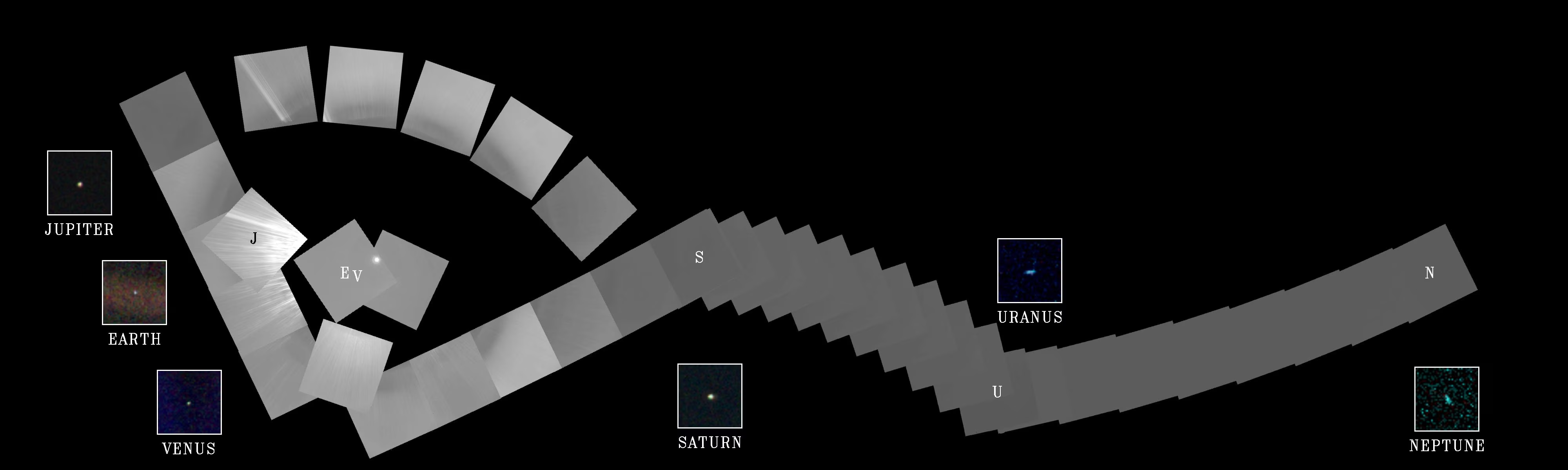
Fig. 11.1 The Voyager 1 “Family Portrait” of the solar system, acquired on 14 February 1990 from roughly 6 billion kilometres distance (PIA00451). Across sixty individual frames spanning roughly 70 degrees of sky, the mosaic captured six planets, including Jupiter, Saturn, Uranus, and Neptune, providing an external view of the planetary system dominated in mass by the gas giants. Credit: NASA/JPL-Caltech.#
Their envelopes are dominated by molecular hydrogen (\(\mathrm{H_2}\)) and helium (He) in near-solar proportions, with slight enrichment in heavier elements (Lecture 2). Neither planet has a solid surface. Pressure and temperature rise smoothly with depth. The gas becomes a supercritical fluid (where liquid and gas become indistinguishable) and then a metallic plasma. By convention, the planetary surface is defined as the level where atmospheric pressure reaches 1 bar [Stevenson, 2020].
Both gas giants rotate rapidly, with periods of about 9 h 56 min for Jupiter and 10 h 33 min for Saturn. Strong Coriolis forces organize atmospheric circulation into alternating east-west bands of bright zones and darker belts. This rapid rotation makes both planets visibly oblate. The flattening is about 6.5% for Jupiter and 9.8% for Saturn. This oblateness constrains the interior density distribution through zonal harmonics (\(J_2, J_4, J_6, \dots\)), gravitational coefficients measured by Juno and Cassini [Iess et al., 2018, Iess et al., 2019].
Both planets radiate more energy than they absorb from the Sun, roughly 1.7 (Jupiter) and 1.8 (Saturn) times the absorbed solar flux. For Jupiter, this excess heat is explained by Kelvin-Helmholtz contraction, the slow planetary contraction releasing gravitational potential energy as heat [Fortney and Nettelmann, 2010]. For Saturn, contraction alone is insufficient. The additional energy comes from helium rain, the immiscibility of helium in metallic hydrogen as droplets settle inward [Stevenson, 1980].
11.1.2. Jupiter interior structure#
Jupiter’s interior consists of fluid layers separated by smooth transitions in composition and physical state [Stevenson, 2020]. Below the molecular \(\mathrm{H_2}\) and He envelope, increasing pressure compresses hydrogen into metallic hydrogen, an electrically conducting state in which electrons become delocalised. This gradual transition occurs near \(100\) GPa and \(5000\) K. That corresponds to a fractional radius of about \(0.85\,R_J\) [Wahl et al., 2017]. Below this depth, the conducting fluid powers the dynamo, the self-sustaining process by which fluid motion generates a magnetic field (Lecture 4), while central conditions reach \(\sim4000\) GPa and \(\sim20{,}000\) K [Militzer et al., 2022, Wahl et al., 2017].
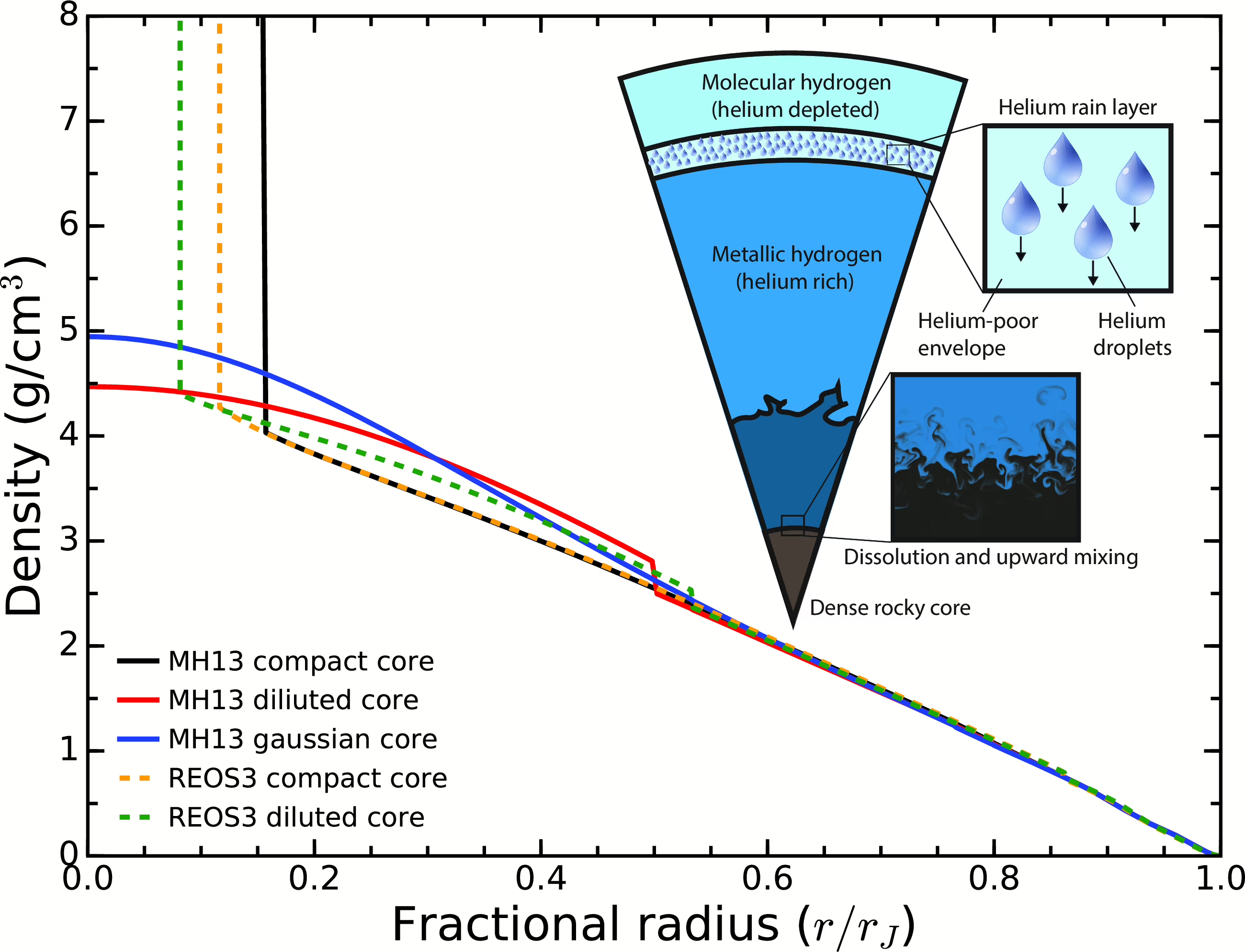
Fig. 11.2 Density as a function of fractional radius for representative Jupiter interior models from Wahl et al. [2017], comparing two equations of state (MH13 and REOS3). The compact-core models (MH13 in black, REOS3 in orange dashed) exhibit a sharp density discontinuity at the inner core boundary near \(r/r_J \approx 0.15\), while the dilute-core models (MH13 in red and blue, REOS3 in green dashed) show a smooth, gradual increase in density across roughly the inner half of the planet. The inset cartoon sketches the layered structure inferred for Jupiter: an outer molecular hydrogen envelope, an intermediate metallic-hydrogen layer with helium-rain droplets, and a dilute core in which heavy elements are mixed throughout the inner region rather than concentrated in a discrete central body.#
Traditional interior models assumed a compact core of heavy elements at fractional radii of less than 0.2, but Juno gravity measurements of zonal harmonics (\(J_4\), \(J_6\), \(J_8\), and \(J_{10}\)) cannot be matched by compact-core models. Instead, the data require a dilute core, in which \(20\text{--}40\,\Mearth\) of heavy elements are distributed across the inner \(30\) to \(50\)% of Jupiter’s radius and smoothly grade into the envelope (Fig. 11.2) [Militzer et al., 2022].
The dilute core has direct implications for planetary formation. A compact core of \(\sim10\,\Mearth\) assembled by core accretion, the formation pathway in which a solid core gravitationally binds a surrounding gas envelope (Lecture 2), is buoyantly stable against mixing and cannot naturally erode into metallic hydrogen. The distributed heavy elements therefore imply either efficient early mixing from a giant impact or the late hydrodynamic accretion of an envelope containing dissolved heavy elements [Militzer et al., 2022].
11.1.3. Jupiter atmosphere and weather#
Jupiter’s visible atmosphere is the cloud-bearing layer between 0.1 and 10 bar. As discussed in Lecture 6, condensation curves set three cloud decks: ammonia ice (\(\mathrm{NH_3}\)) near 0.5 to 1 bar, ammonium hydrosulfide (\(\mathrm{NH_4SH}\)) near 2 to 3 bar, and water ice at \(\sim 5\) to 7 bar. Galileo probe measurements confirmed this layered structure during atmospheric entry in 1995. The entry site was unusually dry, illustrating that local meteorology deviates from horizontally averaged models [Niemann et al., 1998].
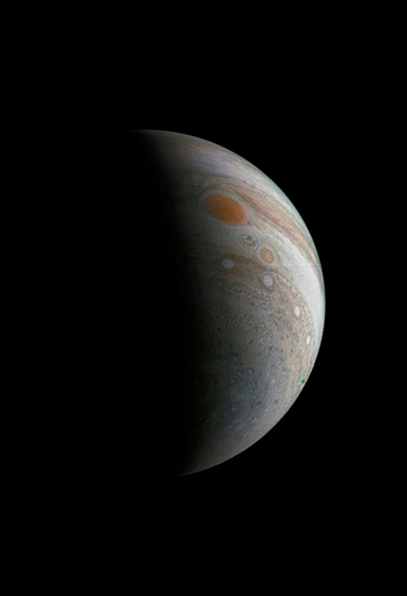
Fig. 11.3 Crescent Jupiter and the Great Red Spot imaged by Juno’s JunoCam during the third close perijove in December 2016. The image is a citizen-science processing of public Juno data and shows the GRS, the train of white ovals known informally as the “string of pearls”, and the long-lived storm Oval BA below the GRS. Image credit: NASA/JPL-Caltech/SwRI/MSSS, processed by Roman Tkachenko.#
About fifteen alternating zonal jets reach velocities of order 180 m s\(^{-1}\) [de Pater and Lissauer, 2010], and bright zones (rising air topped by ammonia clouds) alternate with darker belts (descending air exposing deeper haze). Embedded in this flow is the Great Red Spot (GRS). It is an anticyclonic vortex observed continuously since at least 1830. The GRS has contracted from about 40,000 km at the start of the twentieth century to roughly 14,000 km today. The mechanisms driving this contraction remain debated (Fig. 11.3).
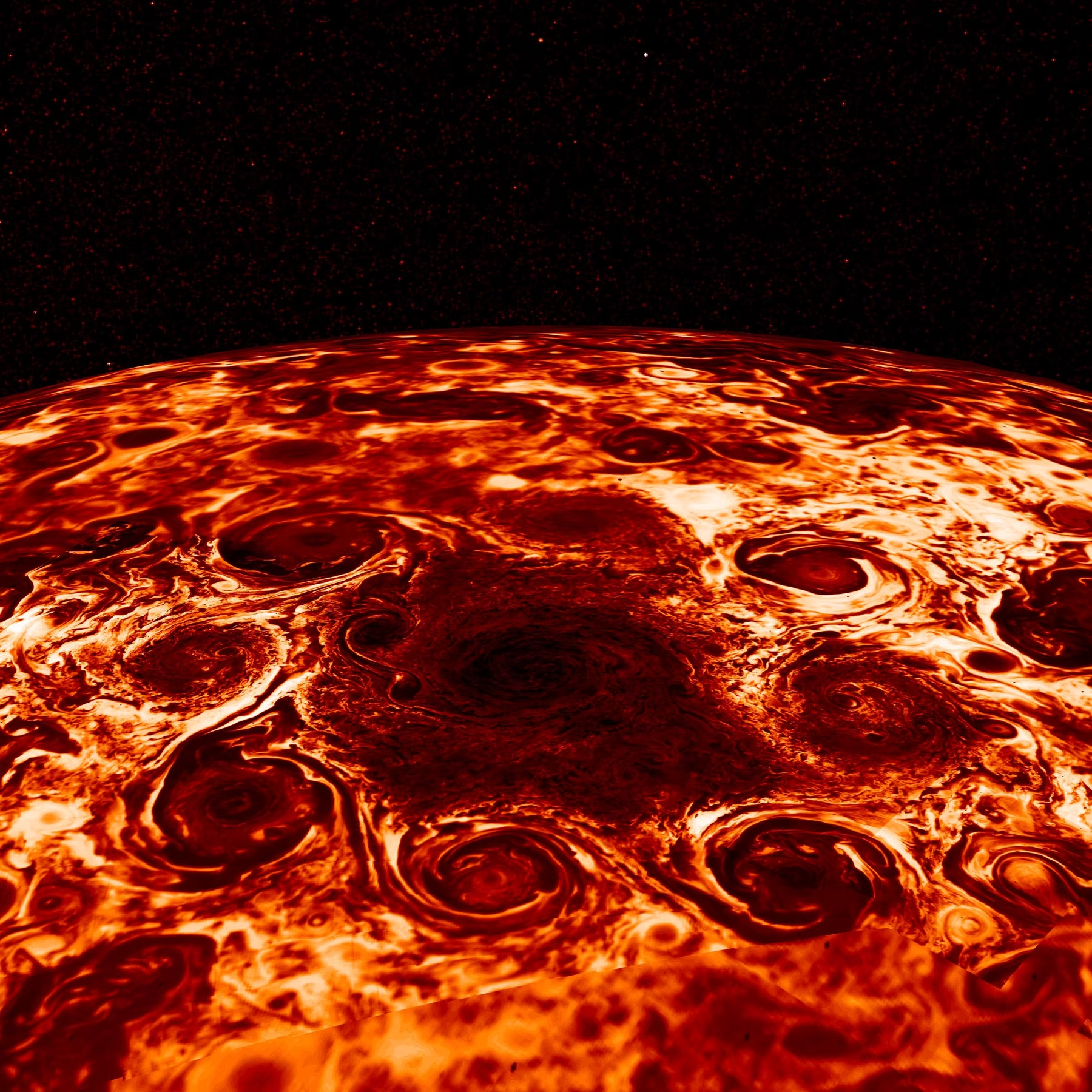
Fig. 11.4 Cluster of cyclones encircling Jupiter’s north pole, imaged by Juno’s JIRAM thermal infrared instrument. A central polar cyclone is surrounded by eight cyclones in a stable polygonal arrangement. The pattern persisted across multiple Juno perijove flybys and demonstrates the rotational organization of Jovian polar weather. Image credit: NASA/JPL-Caltech/SwRI/ASI/INAF/JIRAM. See Adriani et al. [2018].#
Fig. 11.5 shows the cyclone cluster at the south pole.
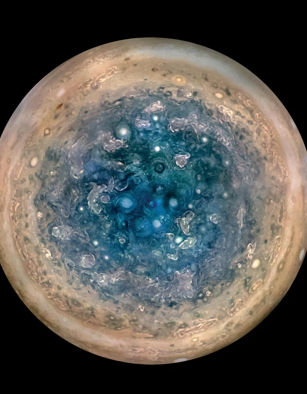
Fig. 11.5 Jupiter’s south pole as seen by JunoCam in visible light. A central cyclone (diameter \(\sim\)5,800 km) is surrounded by five companion cyclones, each \(\sim\)5,600–7,000 km across. Unlike the north pole (where the central cyclone is encircled by eight companions \(\sim\)4,000–4,600 km in diameter), the south pole hosts a pentagonal arrangement, which shows that the polar cyclone clusters are stable but not unique solutions of the deep-jet dynamics. Image credit: NASA/JPL-Caltech/SwRI/MSSS/Betsy Asher Hall/Gervasio Robles. See Adriani et al. [2018].#
Both poles host stable polygonal cyclone clusters: a central cyclone surrounded by eight others at the north pole (Fig. 11.4) and five at the south pole [Adriani et al., 2018]. Kaspi et al. [2018] showed that zonal jets penetrate several thousand kilometres, decaying by \(\sim\)2,000 km and vanishing by \(\sim\)3,000 km, and below this depth magnetic stresses in metallic hydrogen damp differential rotation into solid-body rotation.
Jupiter’s powerful aurorae are driven by magnetospheric processes (Lecture 4) and volcanic mass loading from Io of about \(1\text{ tonne s}^{-1}\) of sulfur and oxygen. Juno also mapped the equatorial “Great Blue Spot”, an intense magnetic anomaly [Connerney et al., 2022].
11.1.4. Io#
Io is the most volcanically active body in the solar system. Its global heat output is about \(10^{14}\) W. This heat is dissipated as tidally driven volcanism rather than radiogenic heat (Lecture 3). It is sustained by tidal flexing in the Laplace resonance, an orbital resonance with Europa and Ganymede (orbital periods 1:2:4) [Peale et al., 1979].
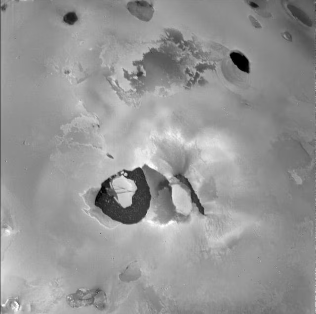
Fig. 11.6 Loki Patera, the largest volcanic depression on Io, imaged by Voyager 1 in 1979. Loki is a periodically resurfacing lava lake about 200 km across that contributes a substantial fraction of Io’s global thermal output. Image credit: NASA/JPL.#
Fig. 11.7 shows an active fire fountain at Tvashtar Catena imaged by Galileo.
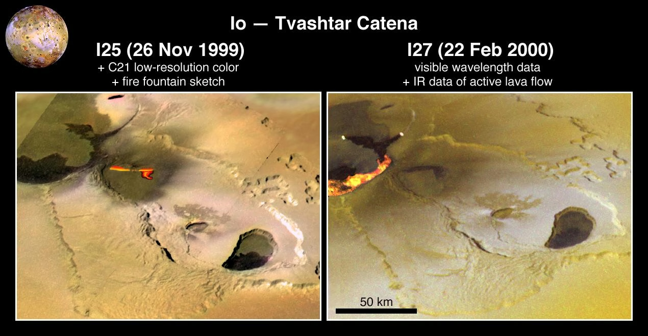
Fig. 11.7 Composite Galileo view of the active fire fountain at Tvashtar Catena on Io, combining low-resolution colour imaging from orbit C21 with visible and infrared data from orbits I25 (26 Nov 1999) and I27 (22 Feb 2000) that captured the active lava flow in the act. Tvashtar is one of the most dramatic active volcanic eruptions documented in the solar system. Image credit: NASA/JPL/University of Arizona.#
Volcanic resurfacing on \(\sim\)Myr timescales leaves Io with essentially no impact craters (Fig. 11.6). Io’s tenuous \(\mathrm{SO_2}\) atmosphere is supplied by volcanic plumes and sublimating surface frosts.
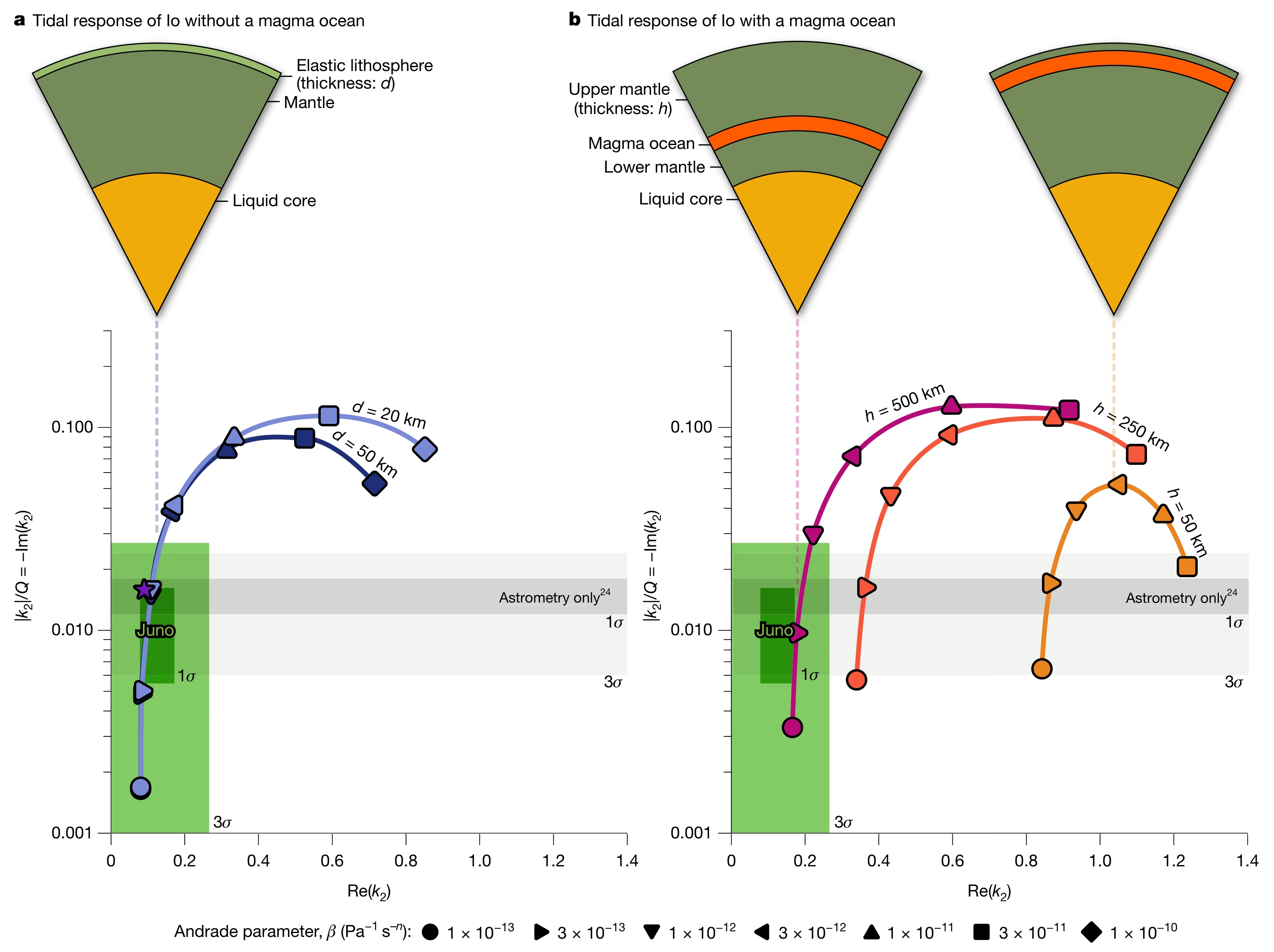
Fig. 11.8 Io’s measured tidal response compared with interior models without (a) and with (b) a global magma ocean. The sketches show the layering of each model. The plots show the dissipation factor \(|k_2|/Q\) (vertical axis, logarithmic) against the real part of the tidal Love number, \(\mathrm{Re}(k_2)\) (horizontal axis). Separate curves correspond to different lithosphere thicknesses \(d\) (a) or to different depths \(h\) of a 100 km thick magma ocean (b); the markers along each curve mark models with different values of the mantle rheology parameter \(\beta\), which sets how strongly the mantle dissipates tidal energy. Green boxes are the 1\(\sigma\) and 3\(\sigma\) Juno constraints, and grey bands mark the earlier astrometry-only constraint. Models without a magma ocean pass through the Juno box for low values of \(\beta\), whereas a magma ocean shallower than about 500 km produces a far larger \(\mathrm{Re}(k_2)\) than measured. The data therefore preclude a shallow magma ocean and are consistent with a mostly solid mantle: a single gravity measurement can rule out a whole class of interior structures. Reproduced from Park et al. [2025].#
Juno measured the gravitational \(k_2\) tidal Love number (a dimensionless measure of tidal deformation) to be \(\mathrm{Re}(k_2) = 0.125 \pm 0.047\) [Park et al., 2025]. This rules out a global shallow magma ocean. It is consistent with a mostly solid silicate mantle with localised partial melting (Fig. 11.8).
11.1.5. Europa#
Europa is an icy Galilean moon (\(R = 1561\) km). Low crater counts indicate a young surface age of 40–90 Myr [Pappalardo et al., 1999]. Its water-ice surface is marked by lineae (long fracture systems) and chaos terrain (disrupted regions of broken and refrozen ice) (Fig. 11.10) (Fig. 11.9).
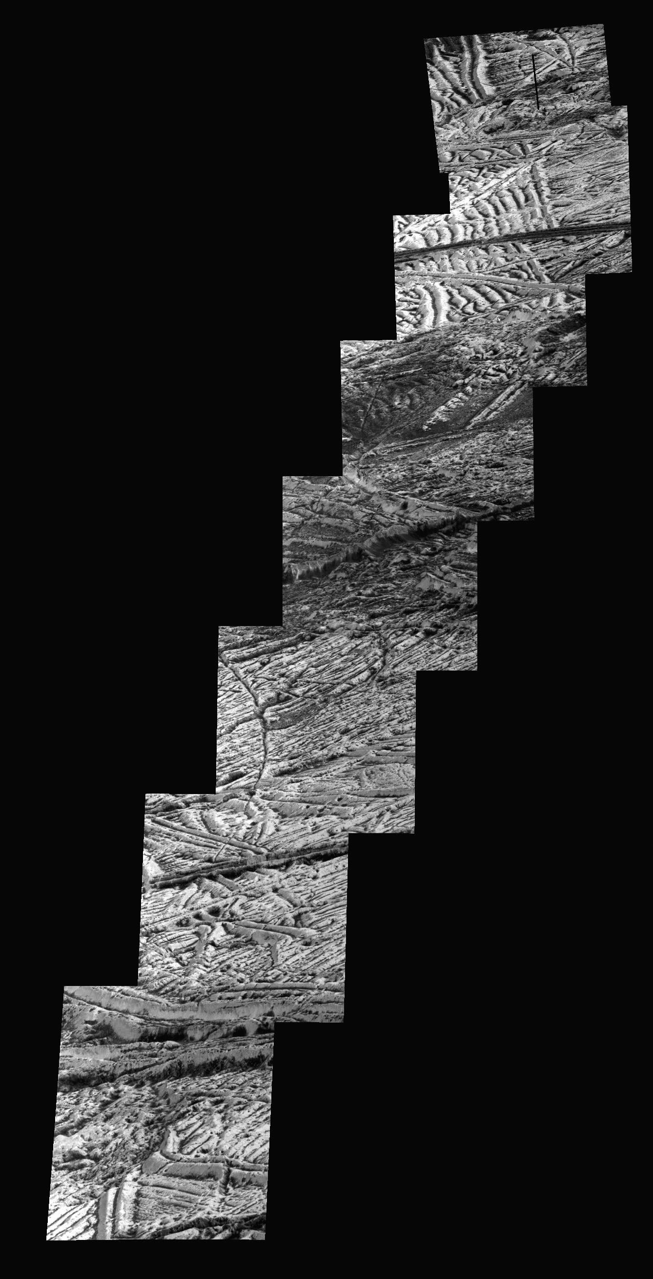
Fig. 11.9 High-resolution view of Europa’s surface from the Galileo orbiter, showing the network of dark and bright lineae (long fractures), patches of chaos terrain, and the limited density of impact craters indicative of a young surface. Image credit: NASA/JPL-Caltech/SETI Institute.#
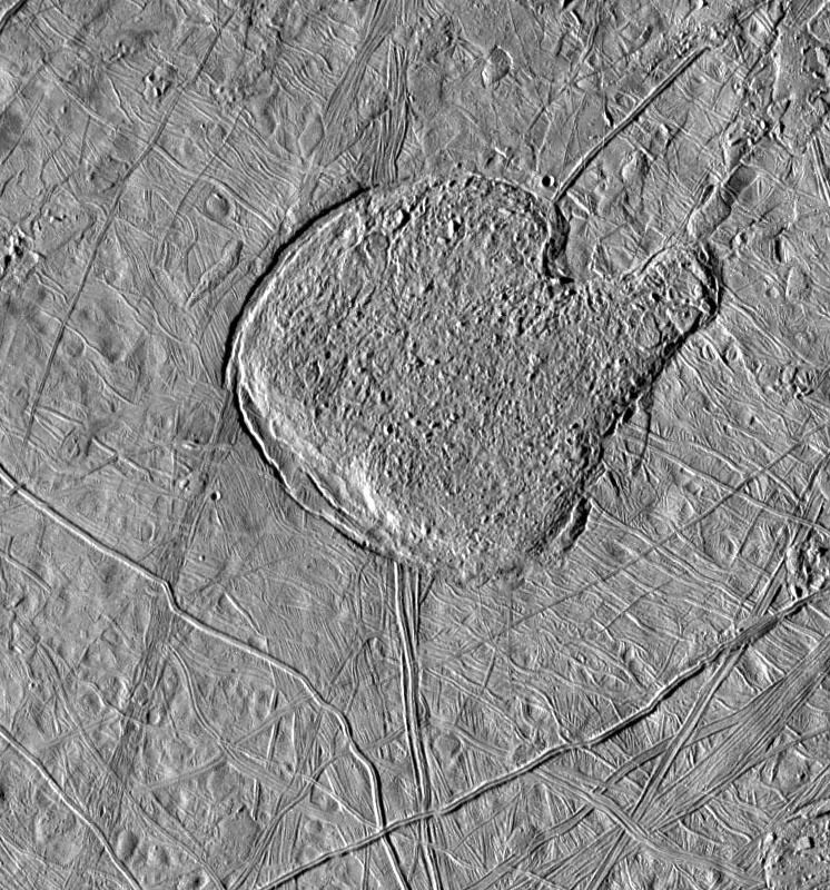
Fig. 11.10 The Conamara Chaos region on Europa imaged at high resolution by the Galileo orbiter (PIA01640). Polygonal blocks of ice have rotated and translated relative to one another and refrozen into a darker matrix material. The morphology is consistent with brief episodes of partial melting and refreezing of the ice shell, possibly driven by warm rising plumes within the ice, by intrusions of ocean water, or by the foundering of slabs of icy crust. Image credit: NASA/JPL-Caltech/ASU.#
Galileo magnetometer data revealed an induced magnetic moment requiring a global, electrically conducting subsurface ocean beneath the ice shell [Khurana et al., 1998]. The ice shell is estimated at 6–25 km thick and the underlying ocean at \(\sim\)100 km deep. This liquid water is sustained by tidal heating generated by Europa’s orbital eccentricity in the Laplace resonance with Io and Ganymede.
NASA’s Europa Clipper mission, launched in October 2024, will arrive at Jupiter in 2030 to conduct approximately fifty close flybys with ice-penetrating radar, a magnetometer, mass spectrometers and high-resolution imaging [Howell and Pappalardo, 2020].
11.1.6. Ganymede#
Ganymede is the largest moon in the solar system. Its radius is 2634 km. It is the only moon with an intrinsic dynamo magnetic field, an internally generated field (Lecture 4, Lecture 8). Its interior is fully differentiated into a metallic iron core, silicate mantle, and outer ice shell (Fig. 11.11) (Fig. 11.12).
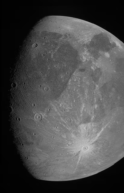
Fig. 11.11 Ganymede imaged by JunoCam during the 7 June 2021 close flyby, the first close encounter with the moon since Galileo’s mission ended in 2003. The image highlights the contrast between bright grooved terrain and darker ancient cratered terrain. Image credit: NASA/JPL-Caltech/SwRI/MSSS.#
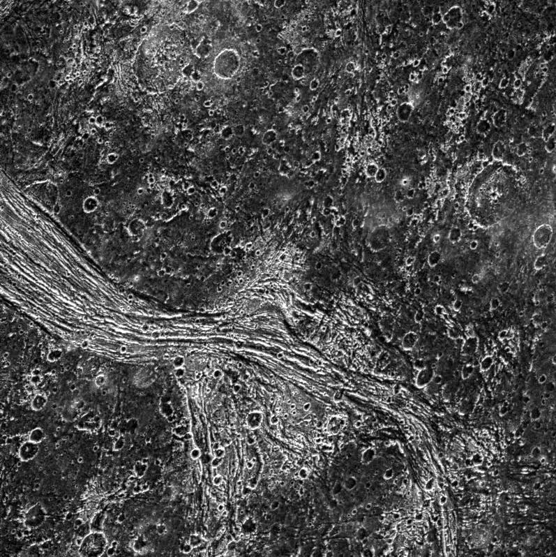
Fig. 11.12 Grooved bright terrain (Lagash Sulcus) cutting through ancient cratered dark terrain in the Marius Regio of Ganymede, imaged at \(\sim\)288 m/pixel by the Galileo orbiter on 6 June 1997 (PIA01617). The parallel ridges and troughs record episodes of tectonic extension early in Ganymede’s history and stand in stark contrast to Callisto’s heavily cratered, undisturbed surface. Image credit: NASA/JPL-Caltech/Brown University.#
Hubble UV observations of auroral rocking require an ocean approximately 100 km deep beneath a 150 km ice shell [Saur et al., 2015]. ESA’s JUICE mission, launched in 2023, will orbit Ganymede in 2034 to map its interior [Grasset et al., 2013].
11.1.7. Callisto#
Callisto, the outermost Galilean moon, is only partially differentiated. Rock and ice are incompletely separated (Fig. 11.14) (Fig. 11.13). Its bulk density of 1834 kg m\(^{-3}\) and dimensionless moment of inertia \(C/MR^2 \approx 0.355\), compared to 0.4 for a uniform sphere, reflect this incomplete separation [Anderson et al., 2001].
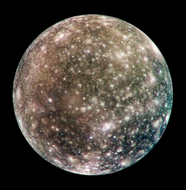
Fig. 11.13 Callisto in global colour view, assembled from Galileo and Voyager images. The surface is dominated by ancient impact craters and lacks the tectonic features that betray subsurface activity on Europa and Ganymede. The bulk density and moment of inertia indicate only partial differentiation. Image credit: NASA/JPL-Caltech.#
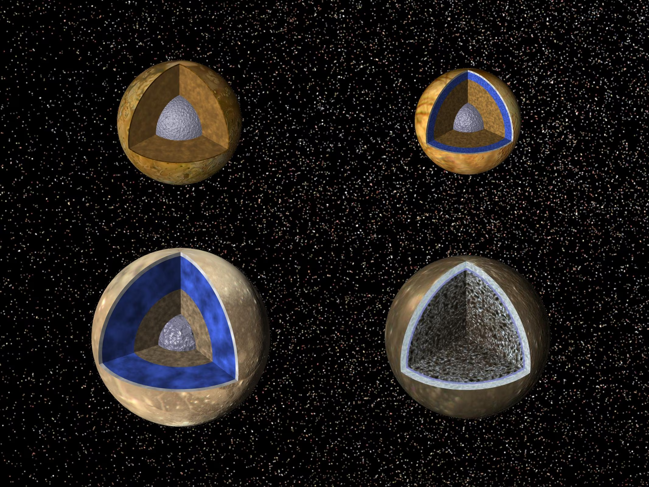
Fig. 11.14 Schematic interior structures of the four Galilean moons (left to right: Io, Europa, Ganymede, Callisto) at comparable scale, NASA/JPL artist concept (PIA01082). Callisto, on the right, is only partially differentiated, in contrast to the fully differentiated Ganymede next to it. Its inferred subsurface ocean (blue layer near the surface) comes from Galileo magnetometer data showing an induced magnetic field similar to that of Europa, although the conducting layer in Callisto is plausibly less massive and less salty. Image credit: NASA/JPL-Caltech.#
Callisto’s heavily cratered surface shows no evidence of tectonic resurfacing. Because Callisto lies outside the 1:2:4 Laplace resonance with Io, Europa, and Ganymede, its eccentricity damps and tidal dissipation is negligible. However, Callisto induces a time-varying magnetic field in the ambient Jovian field, which is most easily explained by a conducting layer near the surface, presumably a salty subsurface ocean [Khurana et al., 1998].
11.1.8. Jupiter’s rings and small moons#
Unlike Saturn’s bright icy rings, Jupiter’s are faint dusty rings (transient debris clouds) ejected from inner moons like Amalthea by micrometeorite impacts (Fig. 11.15).
Atmospheric drag and radiation pressure remove this dust.
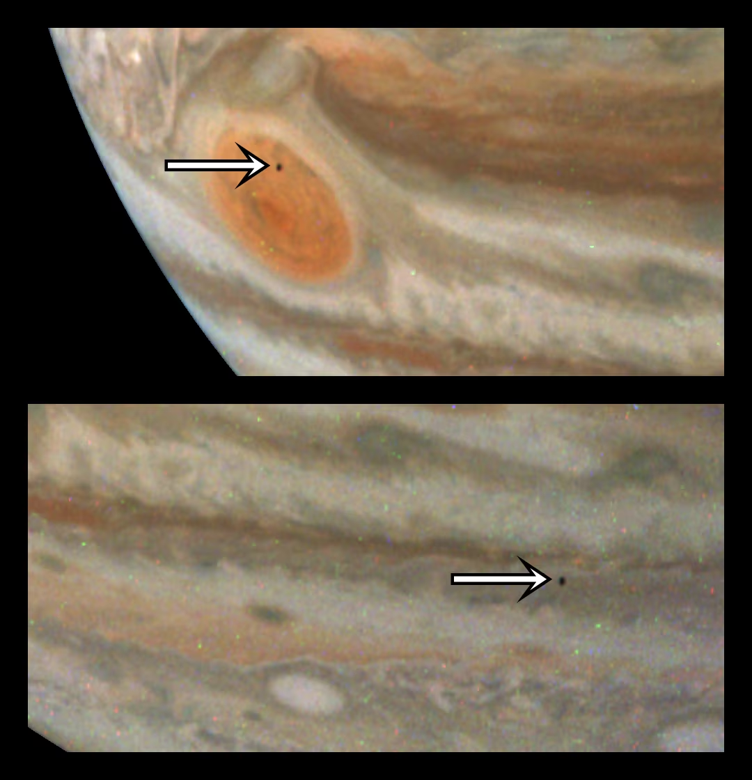
Fig. 11.15 Detection of Amalthea (small silhouette indicated by arrows in both panels) by JunoCam, crossing the Great Red Spot in the top panel and the southern belts in the bottom panel, during the 59th perijove flyby on 7 March 2024 from a distance of \(\sim\)\(265{,}000\) km (PIA25728). Amalthea is unresolved at this geometry: the image documents the moon’s position rather than its shape. Amalthea has a mean radius of \(\sim\)84 km, an irregular shape (\(\sim\)250 \(\times\) 146 \(\times\) 128 km from Galileo data), and a reddish surface believed to reflect contamination from Io’s volcanic plumes; it is one of the principal sources of dust for Jupiter’s faint ring system through micrometeorite gardening of its surface. Image credit: NASA/JPL-Caltech/SwRI/MSSS, processed by Gerald Eichst{“a}dt.#
11.1.9. Saturn interior and rotation#
Like Jupiter, Saturn has a hydrogen and helium envelope. Its lower mass, however, limits the peak interior pressure to a third of Jupiter’s. The metallic hydrogen transition therefore occurs at a smaller fractional radius. Cassini gravity measurements and ring seismology constrain its interior [Mankovich and Fuller, 2021].
At 1 to 3 Mbar and 5000 to 10,000 K, helium becomes immiscible. It forms helium rain: droplets that condense and sink under gravity. Their sinking releases gravitational energy as heat, explaining Saturn’s excess luminosity [Stevenson, 1980]. This process depletes upper-envelope helium, matching Voyager measurements. Jupiter undergoes less helium rain because its hotter interior limits immiscibility.
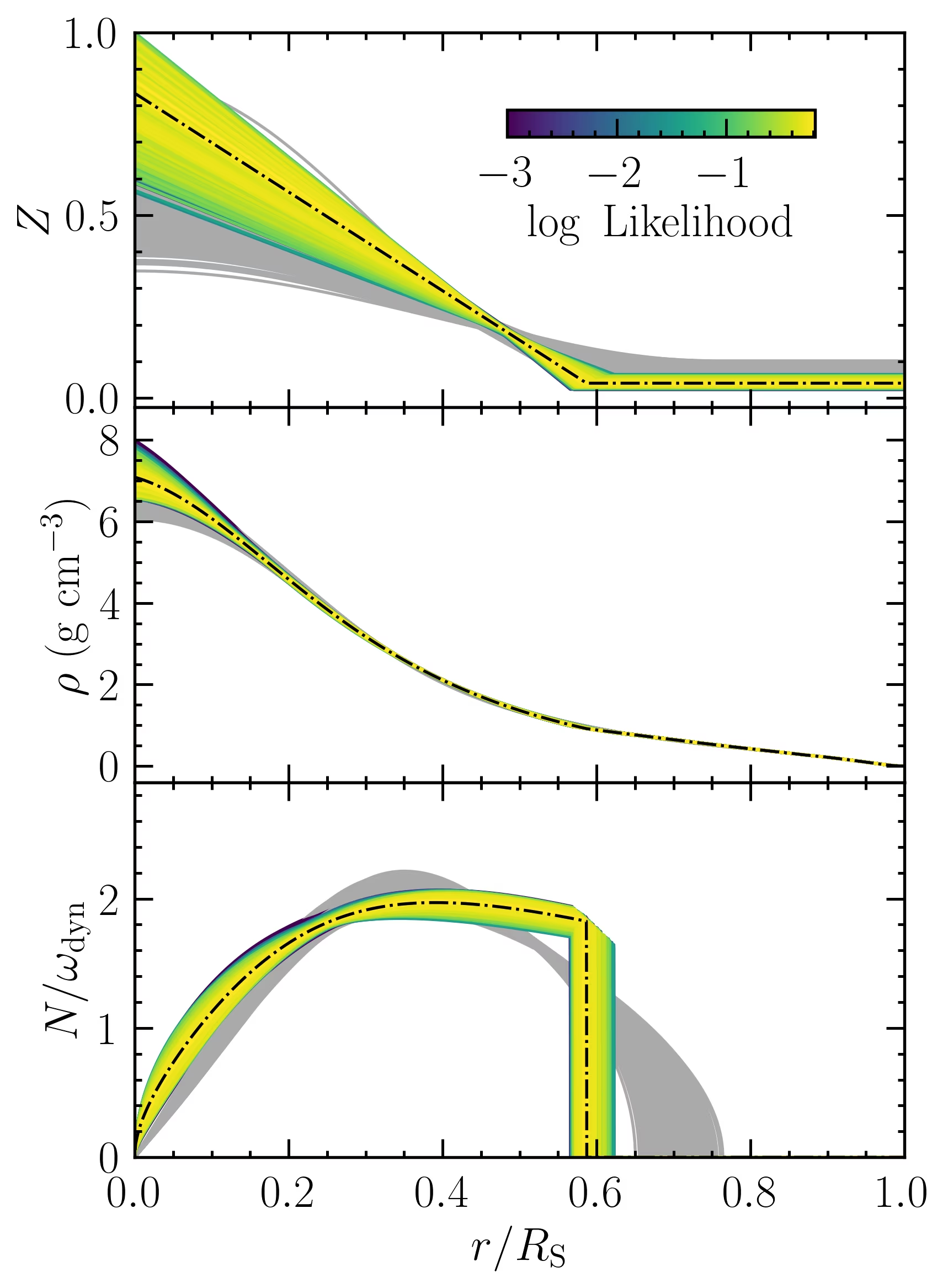
Fig. 11.16 Saturn’s heavy-element distribution \(Z(r)\) (top), density \(\rho(r)\) (middle), and Brunt-Vaisala frequency \(N\) (bottom) as a function of fractional radius from Mankovich and Fuller [2021]. The colour scale is the relative log-likelihood of each model, the yellow track is the maximum-likelihood profile, and the grey envelope is the prior. The heavy elements form a stably stratified, dilute distribution extending out to roughly 60% of Saturn’s radius rather than being concentrated in a compact central core.#
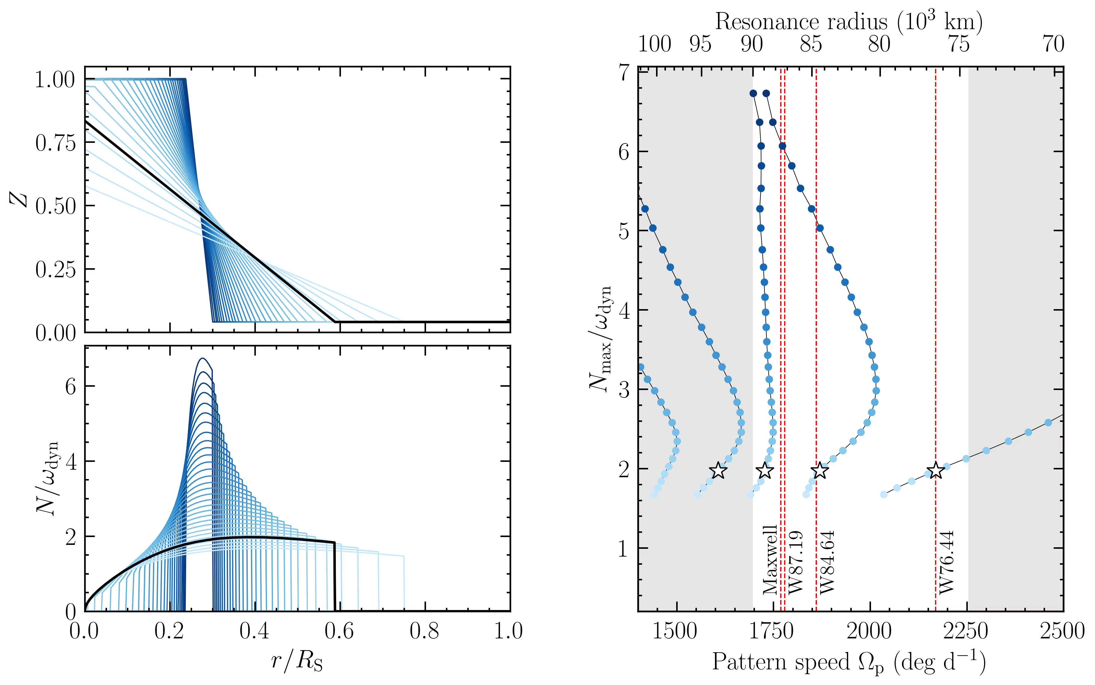
Fig. 11.17 Kronoseismology constraints on Saturn’s interior from Mankovich and Fuller [2021]. Left: family of allowed heavy-element profiles \(Z(r)\) and Brunt-Vaisala frequencies \(N(r)/\omega_{\rm dyn}\). Right: pattern speeds and resonance radii of the f-mode oscillations of Saturn that drive observable density waves in the C ring at \(\sim 75{,}000\)–\(95{,}000\) km radius. The observed waves (red dashed lines, labelled with their ring positions) are reproduced only by interior models with a stably stratified, dilute heavy-element distribution extending to roughly 60% of Saturn’s radius. The figure is the most quantitative external probe of any giant planet interior to date.#
Saturn’s interior is probed by kronoseismology. The method detects f-mode oscillations through C-ring density waves (Fig. 11.17). These waves require a stably stratified, dilute core extending to roughly 60% of Saturn’s radius with \(\sim\)17 \(\Mearth\) of rock and ice (Fig. 11.16) [Mankovich and Fuller, 2021]. Like Jupiter, Saturn has an extended dilute core rather than a compact central core.
Saturn’s rotation period is hard to measure. The reason is that its magnetic dipole aligns with its rotation axis, which suppresses modulated radio emissions. Ring seismology yields the best value: \(10\) h \(33\) min \(38\) s [Mankovich et al., 2019] (Fig. 11.18).
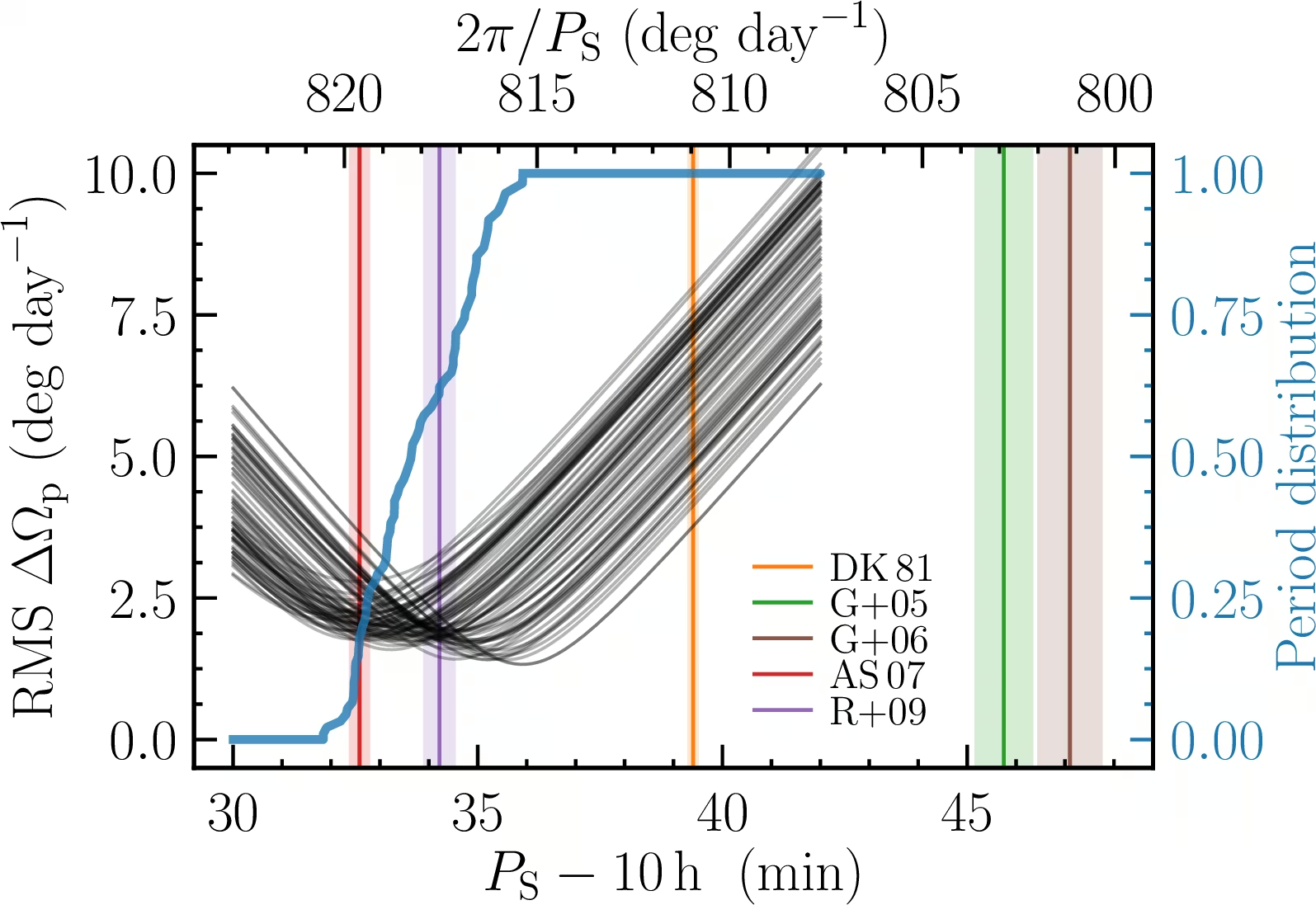
Fig. 11.18 Determination of Saturn’s bulk rotation period from C-ring seismology by Mankovich et al. [2019]. Each black curve shows the RMS pattern-speed residual between an interior model and the set of observed C-ring density waves identified with Saturnian \(f\)-modes, plotted as a function of the assumed rotation period. The thick blue curve gives the cumulative distribution of best-fit rotation periods. The seismological median is \(P_{\rm S} \approx 10\,{\rm h}\,33\,{\rm min}\,38\,{\rm s}\), well separated from the older Voyager and Cassini magnetospheric estimates indicated by the coloured vertical bars.#
A stably stratified helium-rain layer likely filters out non-axisymmetric magnetic fields above the convecting metallic hydrogen, explaining Saturn’s observed axisymmetry despite Cowling’s theorem (Lecture 4).
11.1.10. Saturn atmosphere and weather#
Saturn’s \(\mathrm{NH_3}\), \(\mathrm{NH_4SH}\), and \(\mathrm{H_2O}\) cloud decks parallel Jupiter’s. Yet lower gravity stretches them vertically and lower temperatures push them deeper. Visible contrast across belts and zones is muted, though infrared imaging reveals rich atmospheric texture below the haze.
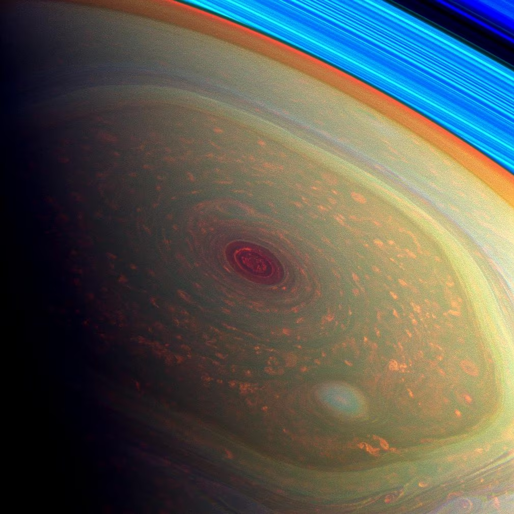
Fig. 11.19 Saturn’s hexagonal polar jet imaged by Cassini, false-colour view (PIA14946). The hexagon, centred at about \(78^\circ\) N, is a standing Rossby wave on a strong eastward zonal jet and has been continuously present since Voyager first observed it in 1981. The false-colour rendering brings out the hexagonal jet boundary that is harder to discern in true-colour imagery. Image credit: NASA/JPL-Caltech/SSI/Hampton University.#
The hexagonal jet stream at \(\sim 78^\circ\) N latitude is a six-sided standing wave observed by Voyager and mapped by Cassini (Fig. 11.19). The hexagon is a Rossby wave locked to an eastward zonal jet. Such a large-scale wave arises because the effective rotation felt by a fluid parcel varies with latitude.
Saturn’s equatorial jet reaches \(\sim\)400 m s\(^{-1}\). Great White Storms are massive convective outbursts. They erupt every \(\sim\)30 years (one Saturnian year) and circle the planet within months. The 2010 to 2011 storm constrained moist convection of water vapour at depth.
11.1.11. Saturn’s rings: structure and composition#
Saturn’s main ring system extends from the D ring at \(\sim\)67,000 km to the F ring at \(\sim\)140,000 km. Arranged radially as D, C, B, A, F, G, and E, the bright A and B rings are separated by the Cassini Division at \(\sim\)118,000 km (Fig. 11.20). The B and C rings lie inside the fluid Roche limit (\(\sim\)126,000 km), while the A ring is bounded by a 7:6 mean-motion resonance with Janus.

Fig. 11.20 Natural-colour radial scan across Saturn’s main rings as imaged by Cassini (PIA08389). The C ring appears as the inner faint band, followed by the bright B ring, the dark Cassini Division at \(\sim\)118,000 km from Saturn’s centre, and the outer A ring. The Cassini Division is maintained by a 2:1 mean-motion resonance with the moon Mimas: ring particles inside the gap are perturbed onto eccentric orbits and are eventually swept out, leaving the gap as a persistent feature. Image credit: NASA/JPL-Caltech/Space Science Institute.#
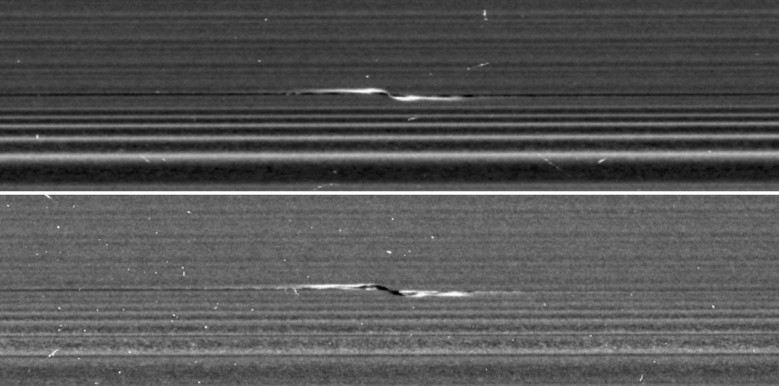
Fig. 11.21 Two close-up Cassini views of the same large “propeller” feature in Saturn’s A ring. The asymmetric S-shape is the gravitational wake carved by an embedded \(\sim\)1 km moonlet that is too small to clear a gap entirely. Tracking these features over the Cassini mission has provided one of the few direct measurements of the orbital evolution of small bodies embedded in a planetary disk [Tiscareno, 2013]. Image credit: NASA/JPL-Caltech/Space Science Institute.#
The rings are composed overwhelmingly of water ice (\(>\)95% by mass), with minor silicates and organics. Particle sizes span 1 cm to 10 m under a power-law distribution. Their vertical thickness is \(\sim\)10 m across \(\sim\)10\(^5\) km radially. The total ring mass is \(\sim\)\(1.5 \times 10^{19}\) kg, about 40% of the mass of Mimas [Iess et al., 2019].
Gravitational interactions with small moons sculpt ring structures. Prometheus and Pandora shepherd the F ring, while Pan clears the Encke Gap in the A ring. A 2:1 mean-motion resonance with Mimas perturbs particle orbits to clear the Cassini Division. Embedded moonlets carve propeller features (partial wakes on either side of their orbit), revealing orbital migration in a planetary disk, the same physics as planet migration in the protoplanetary disc [Tiscareno, 2013] (Lecture 2) (Fig. 11.21).
11.1.12. Saturn’s rings: age and evolution#
Saturn’s rings were long assumed to be primordial (formed at the same time as Saturn 4.5 Gyr ago). Iess et al. [2019] measured a small ring mass from Cassini gravity data, arguing that micrometeorite infall over 4.5 Gyr would have darkened older rings, which favours an age of order \(10^8\) years. However, Crida et al. [2019] showed that viscous evolution from a massive primordial ring can also produce the present-day mass, so mass alone does not uniquely date the rings.
The young-rings hypothesis is supported by direct observations of ring rain (the ongoing transfer of mass from the rings into Saturn’s upper atmosphere). Waite et al. [2018] measured a large flux of water and organic molecules falling into Saturn from the inner D ring during Cassini Grand Finale orbits. Combined with ionospheric \(\mathrm{H_3^+}\) measurements [O'Donoghue et al., 2019], this mass loss indicates a remaining ring lifetime of order \(300\) Myr, with a large uncertainty (\(\sim 170\)–\(1100\) Myr at \(1\sigma\)); the low ring mass and the bright, unpolluted ice independently point to an age of \(\sim 100\) Myr. If correct, Saturn’s rings are temporary (Fig. 11.22).
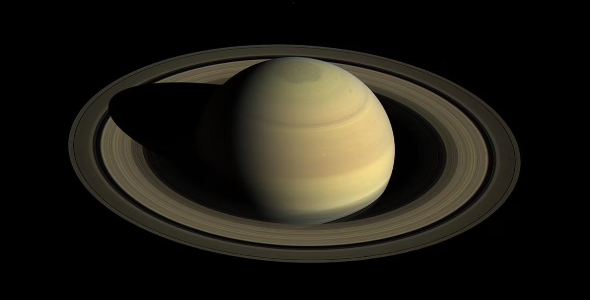
Fig. 11.22 Saturn and its rings imaged by Cassini’s wide-angle camera in April 2016 (PIA21046). The rings are composed almost entirely of water-ice particles whose low mass and high purity indicate an age of order 100 Myr, implying that the ring system may be an ephemeral structure rather than a primordial feature. Credit: NASA/JPL-Caltech/Space Science Institute.#
The ring formation mechanism remains debated. Hypotheses range from recent tidal disruption of an icy moon [Wisdom et al., 2022] to ancient disruption during the Late Heavy Bombardment followed by viscous spreading [Charnoz et al., 2009]. Solar system structures do not all date from 4.5 Gyr ago: dramatic events on \(\lesssim\)Gyr timescales continue to shape what we see today.
11.2. Blackboard derivation: The Roche limit#
Blackboard derivation: The Roche limit
The Roche limit is the orbital distance inside which the tidal field of a primary body exceeds the self-gravity of a fluid satellite, so that the satellite cannot hold itself together gravitationally and is instead disrupted into a disk of particles. The concept was introduced by Roche [1849] and is the key piece of physics behind the existence and location of planetary rings. We derive it here for the simplest case of a fluid (zero-strength) satellite of uniform density.
Setup. Consider a planet of mass \(M_p\), radius \(R_p\), and density \(\rho_p\). A small spherical satellite of mass \(M_s\), radius \(R_s\), and density \(\rho_s\) orbits at distance \(d\) from the planet’s centre, with \(d \gg R_s\) so that we can use a leading-order Taylor expansion of the planet’s gravitational potential across the satellite. We work in the satellite’s rest frame and ask: at what distance \(d\) does the planetary tide stretch the satellite’s surface elements faster than the satellite’s own gravity can pull them back?
Fig. 11.23 shows the setup: the planet on the left, the satellite at distance \(d\), and the two gravitational accelerations whose difference is the tide.
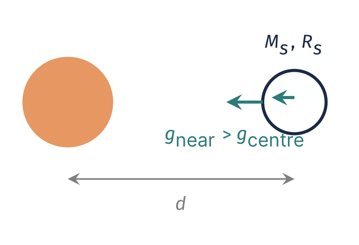
Fig. 11.23 Setup sketch of the board derivation of the Roche limit: planet \(M_p\) and a uniform fluid satellite of mass \(M_s\) and radius \(R_s\) at distance \(d\); the planet’s pull on the satellite’s near side, \(g_{\mathrm{near}}\), exceeds the pull on its centre, \(g_{\mathrm{centre}}\), and this difference stretches the satellite. Course-original figure.#
Step 1: Tidal acceleration across the satellite. The gravitational acceleration from the planet at the satellite’s centre is
At the point on the satellite’s surface closest to the planet, at distance \(d - R_s\), the planetary acceleration is
The differential acceleration across the satellite, that is, the tidal acceleration that tends to stretch the satellite along the planet-satellite line, is
Expanding to first order in the small quantity \(R_s/d\),
so the tidal acceleration becomes
This is the standard result that tidal forces fall off as \(d^{-3}\) rather than \(d^{-2}\).
Step 2: Self-gravity at the satellite’s surface. For a uniform satellite of density \(\rho_s\), the gravitational acceleration at its surface is
Step 3: Setting the two equal. The Roche limit corresponds to the distance at which the tidal stretching just overcomes self-gravity, \(\Delta a_{\rm tidal} = a_{\rm self}\):
Cancel \(G\) and \(R_s\), and substitute \(M_p = (4/3)\pi R_p^3 \rho_p\):
which simplifies to
This is the rigid-body Roche limit: the minimum orbital distance at which a satellite held together only by its own gravity, treated as a rigid sphere, can survive without surface elements being pulled away.
Step 4: The fluid Roche limit. A more careful analysis for a fluid satellite, which deforms into an elongated ellipsoid before disruption rather than remaining spherical, was first carried out by Roche himself [Roche, 1849]. The fluid case is analytically much more involved because it requires solving for the equilibrium shape of a self-gravitating fluid in a tidal field, but the result is that the prefactor changes from \(1.26\) to roughly \(2.46\):
The rigid-body case underestimates the critical distance because it ignores the additional stress imposed by the tidal deformation itself. For most realistic cases, including ice or rock satellites, the answer lies between the two extremes.
Step 5: Application to Saturn’s rings. Saturn has equatorial radius \(R_p = 60{,}268\) km, but for the Roche calculation we use the volumetric mean radius \(R_p \approx 58{,}232\) km (which is the spherical-equivalent value entering the bulk-density definition \(\rho_p = M_p/(4\pi R_p^3/3) = 687\) kg m\(^{-3}\)). For ring particles dominated by water ice, \(\rho_s \approx 1000\) kg m\(^{-3}\), so
This matches the observed outer edge of the A ring (at \(\sim 137{,}000\) km) to within \(\sim\)10%, the discrepancy being plausibly accounted for by the finite material strength of cold ice (which gives the satellite a non-zero rigidity), by the fact that the ring particles have lower density than pure ice because they are porous, and by the density wave structure at the very edge of the A ring. The faint G ring at \(\sim\)170,000 km lies outside the formal Roche limit; it is held together by the small moon Aegaeon embedded within it rather than by self-gravity.
The physical interpretation is that, interior to \(d_R\), the differential pull of the planet across any solid agglomerate is so strong that the agglomerate cannot grow above \(\sim\)\(10\) m without being torn apart. Ring particles therefore orbit as a collisional disk maintained by mutual scattering rather than as a single coalesced moon. This is the key explanation for why rings exist where they do: not because anything special happened locally, but because tidal forces inside the Roche limit forbid the particles from doing what they would otherwise do, namely accrete into a single body.
Fig. 11.24 compares differential tidal acceleration with self-gravity across orbital distance and illustrates the deformation of a fluid satellite at the Roche limit.
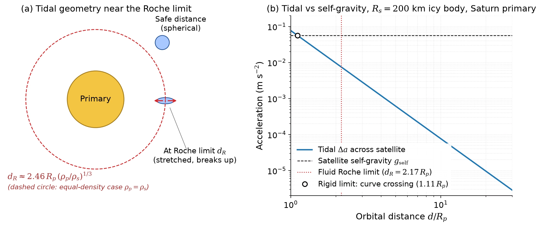
Fig. 11.24 Roche limit geometry and tidal force balance. (a) A self-gravitating fluid satellite deforms into an elongated ellipsoid before disruption at the Roche limit \(d_R\), where differential tidal acceleration overcomes its self-gravity. (b) Differential tidal acceleration across an icy body compared with its surface self-gravity as a function of orbital distance from Saturn; the curves cross at the rigid Roche limit, while the fluid Roche limit accounts for tidal elongation. Course-original figure.#
11.3. Saturn’s moons#
11.3.1. Titan#
Titan (\(R = 2575\) km) is Saturn’s largest moon. It is the only moon in the solar system with a substantial atmosphere. Cassini and Huygens explored it during a 13-year tour and an atmospheric descent in January 2005.
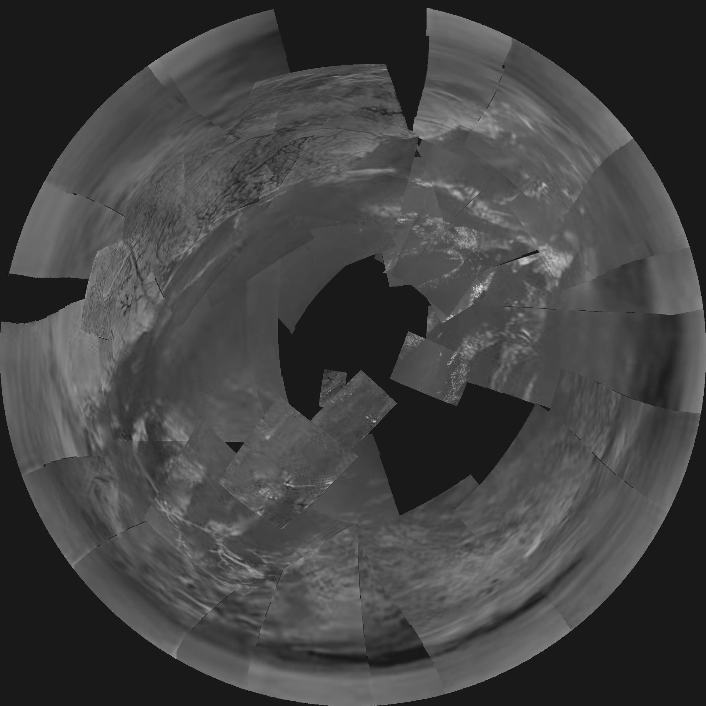
Fig. 11.25 Stereographic projection mosaic of Huygens DISR descent images, taken on 14 January 2005 from an altitude of \(\sim\)3 km above Titan’s surface (PIA07870). The brighter, elevated terrain at top is criss-crossed by dendritic drainage channels carved by methane runoff, which empty into a darker, flatter region resembling a coastline with offshore “islands” and shoals. The methane hydrology of Titan was confirmed in situ for the first time. Image credit: ESA/NASA/JPL-Caltech/University of Arizona.#
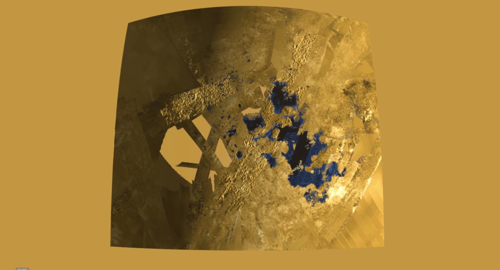
Fig. 11.26 Lakes and seas of liquid methane and ethane near Titan’s north pole, mapped by the Cassini RADAR instrument. The dark patches are radar-smooth liquid surfaces. Ligeia Mare and Kraken Mare are the largest, comparable in size to the Caspian Sea. Image credit: NASA/JPL-Caltech/ASI/Cornell.#
Titan’s \(\mathrm{N_2}\) atmosphere has a surface pressure of 1.5 bar and a temperature of \(\sim\)94 K; the cold makes the surface air density (\(\sim\)5 kg m\(^{-3}\)) about four times that of Earth’s near-surface air. Near its triple point at 94 K, methane (\(\mathrm{CH_4}\)) drives an active hydrological cycle of rain and river channels (Lecture 6) [Stofan et al., 2007] (Fig. 11.25). Cassini RADAR mapped polar liquid hydrocarbon lakes including Kraken Mare and Ligeia Mare (Fig. 11.26).
Solar ultraviolet radiation breaks \(\mathrm{CH_4}\) apart. The products include HCN, \(\mathrm{C_2H_2}\), \(\mathrm{C_2H_4}\), and \(\mathrm{C_2H_6}\). These condense into tholins, solid aerosol particles that produce Titan’s orange haze and settle into dunes. This haze obscures the surface in visible light. Observers need infrared windows and radar.
Cassini gravity and tidal measurements established a global subsurface ocean beneath an ice shell of order 100 km thick [Iess et al., 2012]. Titan therefore joins Europa, Ganymede, Callisto, and Enceladus as an ocean world. Surface organics above a subsurface ocean make Titan a prime astrobiology target.
NASA’s Dragonfly rotorcraft, scheduled for launch in 2028 and arrival in 2034, will fly in Titan’s dense atmosphere to sample surface organics and prebiotic chemistry [Lorenz et al., 2018].
11.3.2. Enceladus#
Enceladus is a small moon of 252 km radius. In 2005, Cassini discovered active geysers erupting from south polar fractures called tiger stripes [Porco et al., 2006] (Fig. 11.29) (Fig. 11.27).
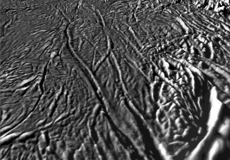
Fig. 11.27 The “tiger stripes” of Enceladus: four parallel fracture zones near the south pole that are the source regions of the active plumes. The fractures are warmer than the surrounding terrain by tens of kelvins, and their ages and orientations track the stress field induced by Enceladus’s eccentric orbit around Saturn. Image credit: NASA/JPL-Caltech/SSI.#
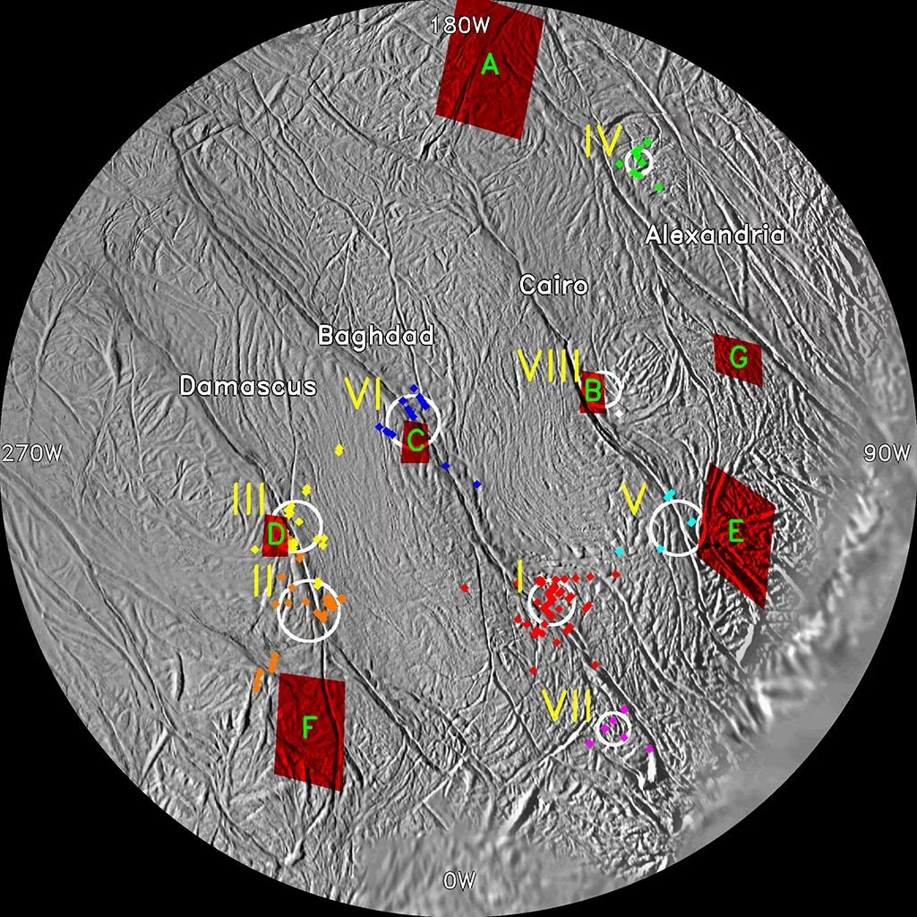
Fig. 11.28 Map of Enceladus’s south polar region showing the correlation between jet sources identified in Cassini imaging (coloured diamonds; white circles indicate location uncertainty) and the hot spots located along the four “tiger stripe” fractures by Cassini’s Composite Infrared Spectrometer (CIRS) (PIA08385). The jets erupt from the warmest portions of the fractures, which are tens of kelvins warmer than the surrounding terrain. The localised heat output is essential evidence that tidal heating is concentrated at the fracture system rather than distributed across the whole moon. Image credit: NASA/JPL-Caltech/GSFC/SwRI/SSI.#
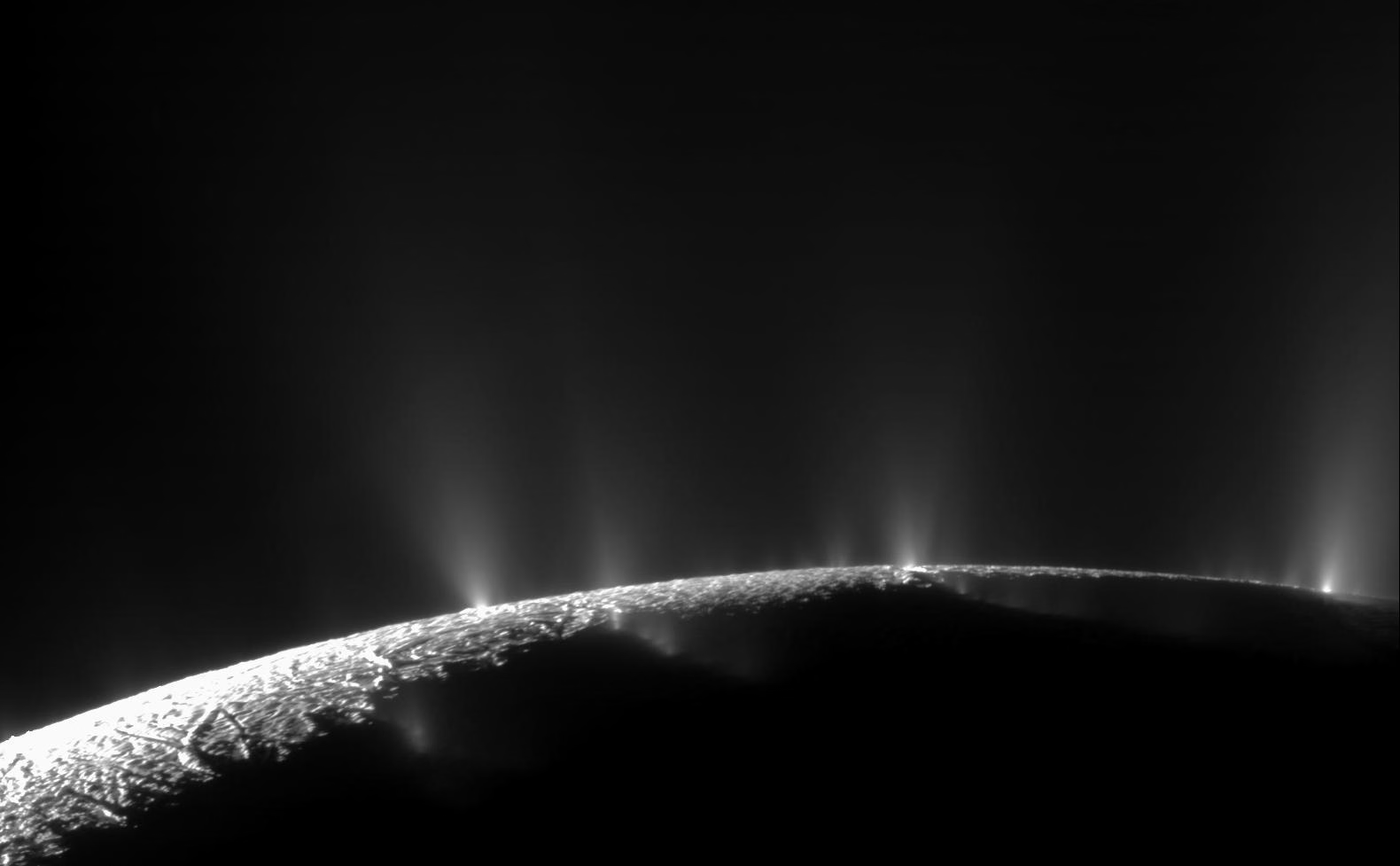
Fig. 11.29 Cassini image of dozens of individual geyser jets erupting from the tiger stripes of Enceladus, observed against a dark background. The plumes deposit material into Saturn’s E ring and feed the magnetospheric plasma with water-group ions. Image credit: NASA/JPL-Caltech/SSI.#
The plumes contain water vapour (about 90%), salts (NaCl, KCl), and organic molecules. Detection of \(\mathrm{H_2}\) is consistent with serpentinisation, water-rock reactions at the seafloor [Waite et al., 2017]. Phosphates and silica nanoparticles imply hydrothermal activity and the presence of biochemical building blocks [Postberg et al., 2023].
A global ocean lies beneath an ice shell of 20 to 30 km. The shell thins at the south pole. A 2:1 mean-motion resonance with Dione drives tidal heating concentrated at the south pole (Fig. 11.28). There, heat flow exceeds 10 GW.
Water, rock contact, energy, and organics make Enceladus a prime candidate for habitability, with biosignature criteria explored in Lecture 14.
11.3.3. Other Saturnian moons#
Saturn’s mid-sized moons form a comparative laboratory. Mimas is dominated by the 130 km Herschel crater on a 200 km radius moon (Fig. 11.30). Evidence for a subsurface ocean is contested.
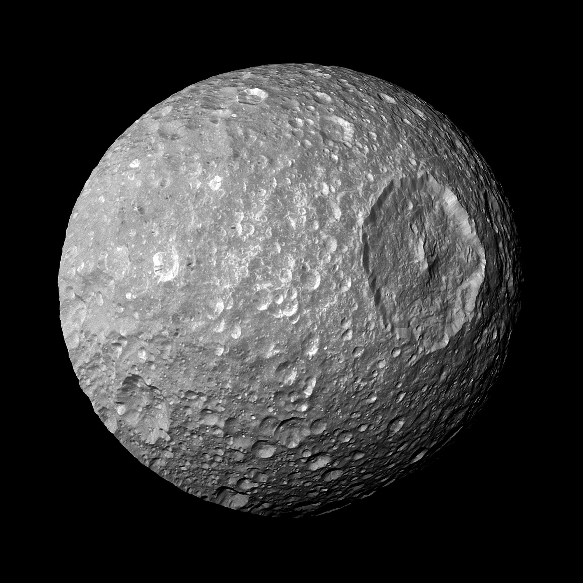
Fig. 11.30 Mimas dominated by the giant Herschel impact crater, imaged by Cassini during its 13 February 2010 close flyby. The crater is \(\sim\)130 km across on a moon with mean radius \(\sim\)200 km, and the impact that formed Herschel was probably close to the catastrophic disruption threshold. Image credit: NASA/JPL-Caltech/Space Science Institute.#
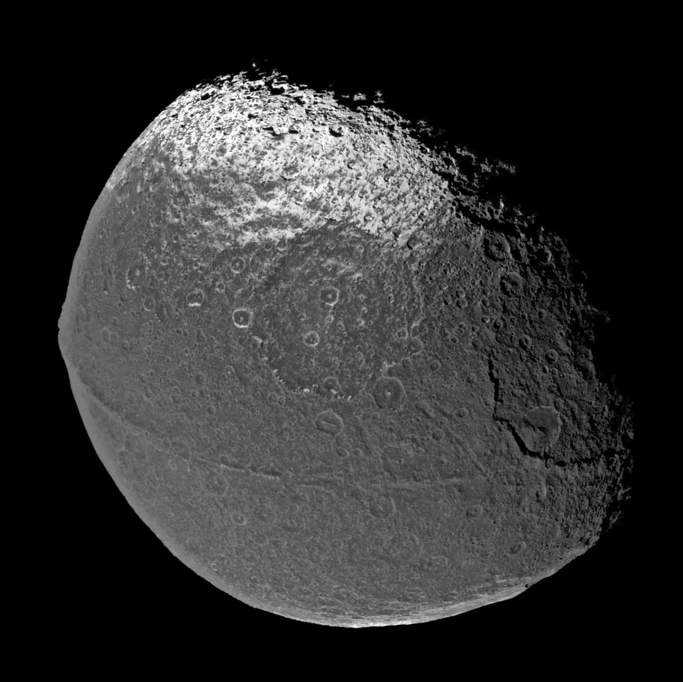
Fig. 11.31 Iapetus showing the two-toned hemispheric pattern, Cassini global mosaic from the 31 December 2004 flyby (PIA06166). The leading hemisphere (the dark Cassini Regio, covering nearly the entire visible disc here) is coated with material believed to be infall from the distant outer retrograde moon Phoebe, while the trailing hemisphere is bright water ice. A thermal-segregation feedback amplifies the contrast: the dark side absorbs more sunlight, gets warmer, sublimates ice, and becomes darker still, while the bright side stays cold and accumulates frost. The narrow ridge running along the equator is also visible. Image credit: NASA/JPL-Caltech/Space Science Institute.#
Fig. 11.32 shows Phoebe, the captured outer moon whose dark infall coats the leading hemisphere of Iapetus.
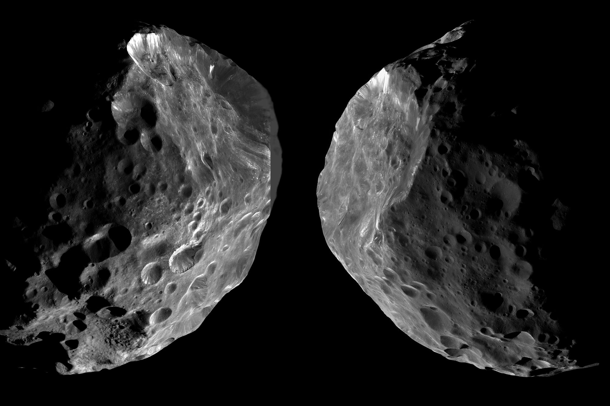
Fig. 11.32 Phoebe, an outer irregular moon of Saturn, meaning its distant, retrograde, and highly inclined orbit marks it as captured rather than formed in place around the planet. Phoebe is widely interpreted as a captured Kuiper Belt object and is the source of dark dust that infalls onto Iapetus’s leading hemisphere. Image credit: NASA/JPL-Caltech/Space Science Institute.#
Iapetus has a dark leading hemisphere coated by infall from Phoebe and a bright icy trailing hemisphere. The contrast is amplified by thermal segregation: dark material absorbs sunlight, sublimating ice onto the colder bright side. It also features a \(\sim\)20 km high equatorial ridge (Fig. 11.31).
Hyperion is a chaotic rotator, while distant retrograde Phoebe represents a captured Kuiper Belt object (Lecture 12).
Tethys, Dione, and Rhea show variable cratering and tectonism at intermediate sizes, and they illustrate how size, distance, and orbital history govern tidal heating and ocean retention.
11.4. Part 2: The ice giants, Uranus and Neptune#
11.4.1. Ice giant overview: the exotic twins#
Uranus (\(14.5\,\Mearth\), \(4.0\,\Rearth\)) and Neptune (\(17.1\,\Mearth\), \(3.9\,\Rearth\)) are ice giants, planets whose bulk composition is distinct from the gas giants [NASA Jet Propulsion Laboratory, 2026]. Hydrogen and helium envelopes account for only \(\sim\)10 to 20% of their mass. The bulk, by contrast, consists of “ices”: water, ammonia, and methane. These “ices” are dense fluids at interior conditions; the name records their origin as solid grains in the outer protoplanetary disk [Helled et al., 2020]. Fig. 11.33 shows how little the gravity data constrain the arrangement of these materials inside the two planets.
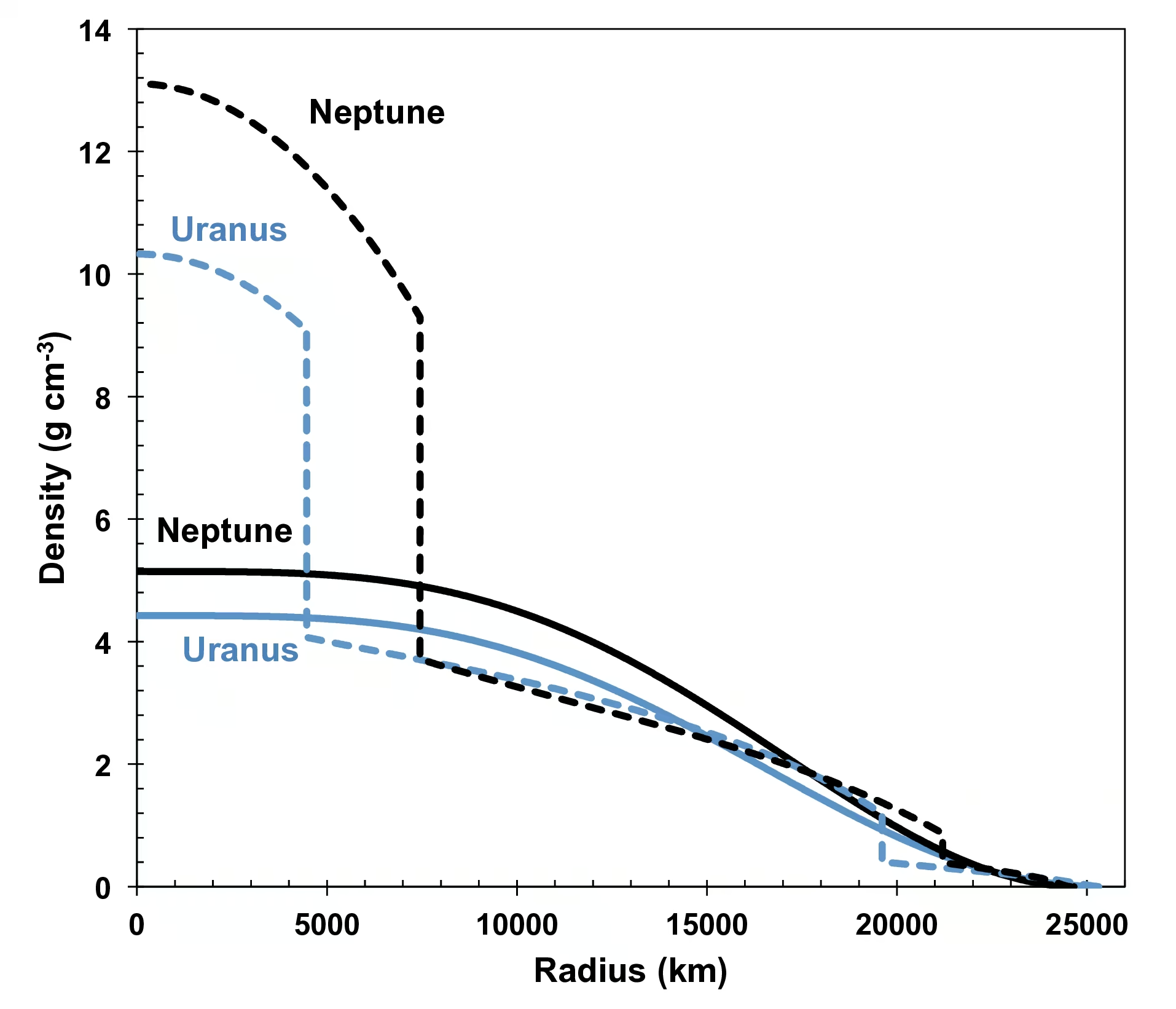
Fig. 11.33 Density as a function of radius for Uranus (blue) and Neptune (black) from Helled et al. [2020]. Solid curves are the empirical density profiles derived in earlier work, dashed curves are three-layer models with discrete envelope, ice, and rock layers. The two profiles match the gravity data equally well, which shows the strong degeneracy between smooth and layered interior models that prevents us from uniquely identifying the bulk composition of the ice giants. Reproduced from Helled et al. [2020].#
Both planets were visited by only one spacecraft, Voyager 2, which flew past Uranus in January 1986 and Neptune in August 1989 [Stone and Miner, 1989]. With no return mission in 35 to 40 years, the ice giants remain the most under-explored major planets. Detailed knowledge of their atmospheres, magnetic fields, and satellites comes from these flybys, supplemented by ground-based, Hubble, and JWST observations [de Pater et al., 2022].
11.4.2. Uranus: the tilted planet#
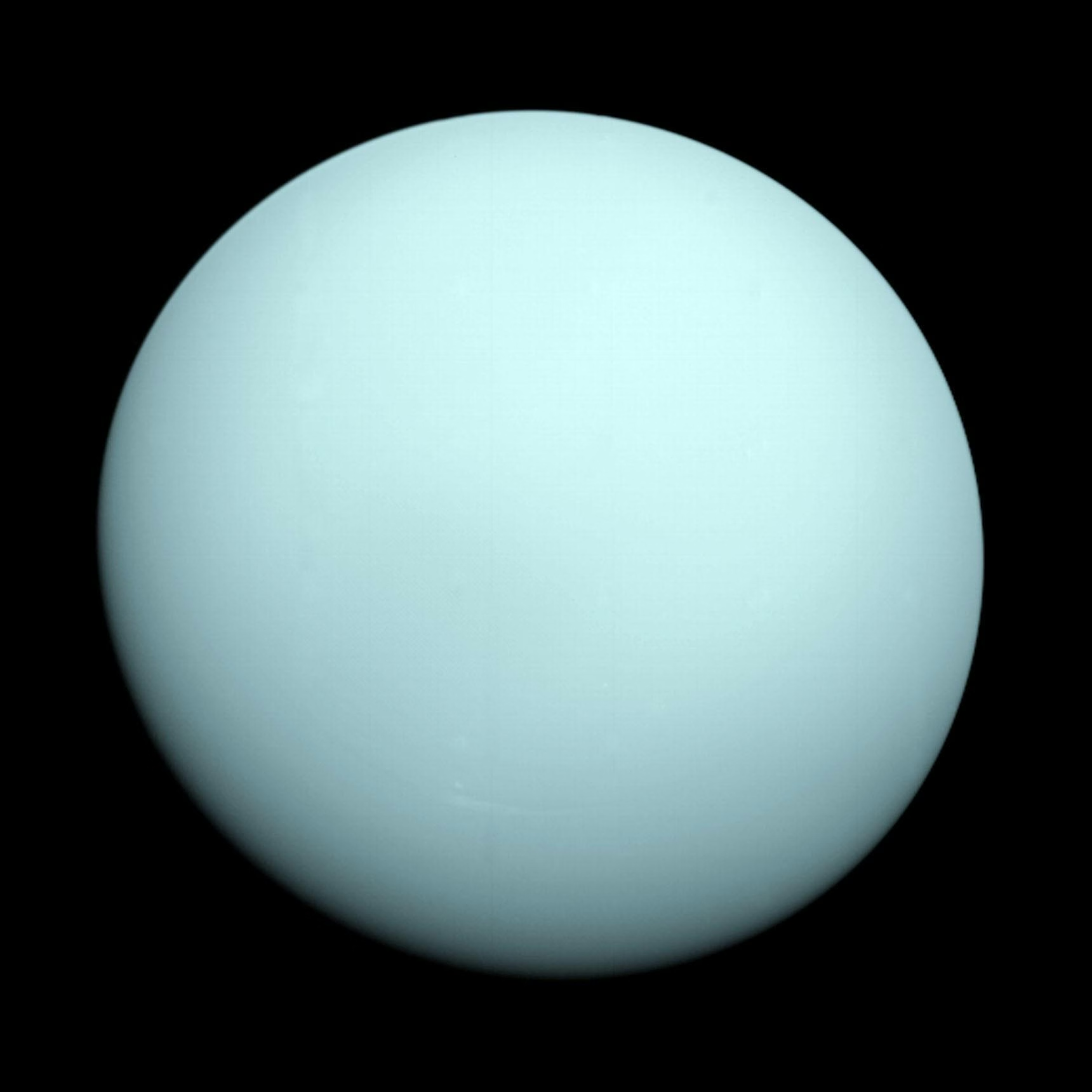
Fig. 11.34 Uranus as seen by Voyager 2 in 1986. The planet appeared remarkably featureless at the time of the flyby, a consequence of being seen near solstice with one pole pointing nearly toward the Sun. Image credit: NASA/JPL-Caltech.#
Uranus has an axial tilt of \(97.8^\circ\). Its rotation axis lies almost in the orbital plane. Over its 84-year orbit, each pole experiences 42 years of continuous daylight followed by 42 years of darkness. At least two giant impacts, an earlier partial tilt and a final oblique one, likely produced the tilt and spun up an equatorial debris disk from which regular satellites re-accreted (Fig. 11.35) [Morbidelli et al., 2012].
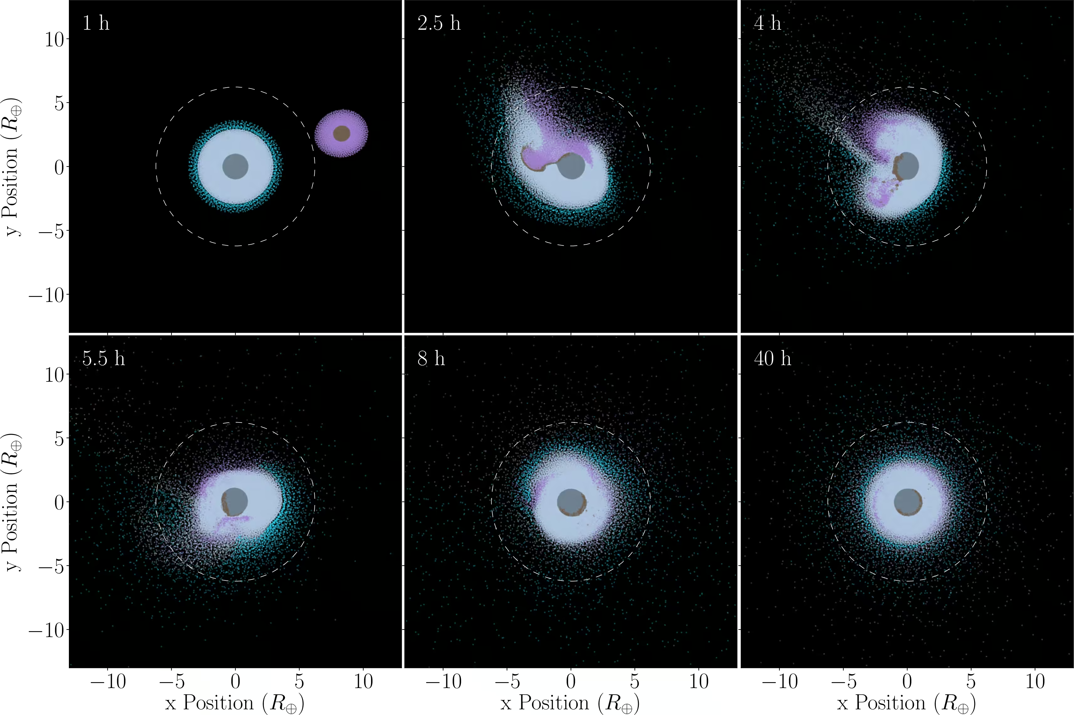
Fig. 11.35 Smoothed-particle-hydrodynamics simulation of a giant impact on the proto-Uranus, from Kegerreis et al. [2018]. Snapshots are shown from \(t = 1\) h to \(t = 40\) h after first contact for a \(2\,\Mearth\) impactor on a low angular momentum trajectory. Particles are coloured by material and origin: light and dark grey are target ice and rock, light blue is target H/He atmosphere, and purple and brown are the corresponding impactor materials. The white dashed circle marks Uranus’s present-day Roche radius. Such oblique collisions deliver enough angular momentum to tilt the proto-Uranus’s spin axis by tens of degrees, can deposit impactor rock into the deep interior, and (for higher angular momentum cases) eject a debris disk in the new equatorial plane from which the regular Uranian satellites later re-accrete. ```During the 1986 Voyager 2 flyby near solstice, Uranus appeared featureless with its south pole pointing toward the Sun (Fig. 11.34). Since the 2007 equinox, as northern summer approaches, observations have revealed increasing cloud activity, including storms in 2014, a polar cyclone, and distinct polar cap structure [de Pater et al., 2022].#
Uranus has an anomalously low internal heat flow. It radiates only 1.06 times the absorbed solar flux [Pearl et al., 1990]. By contrast, Neptune radiates 2.6 times the absorbed flux despite being further from the Sun. This suppressed heat loss may result from a stratified interior that inhibits convective cooling, from deep latent heat release, or from a late perturbation that reset the thermal history. None of these explanations is confirmed. A dedicated Uranus orbiter would be the most direct test.
Neptune: the active ice giant
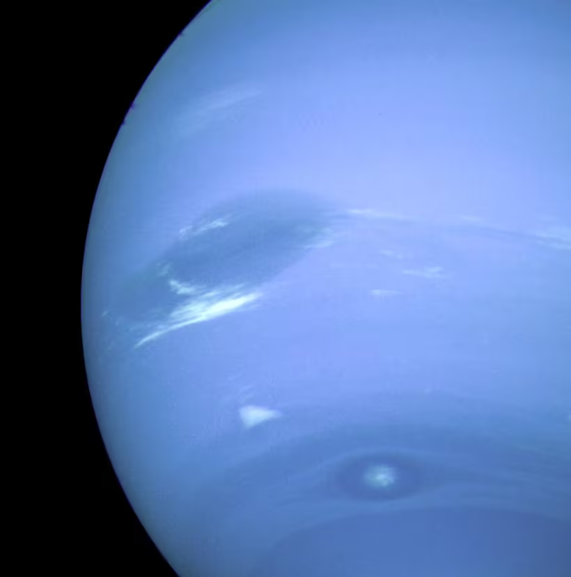
Fig. 11.36 The Great Dark Spot of Neptune (centre left), an anticyclonic storm in the southern hemisphere, imaged by Voyager 2 in August 1989. It was comparable in size to Earth and was bordered by bright methane cirrus clouds; a second dark storm, Dark Spot 2, lies at lower right. The small bright cloud below the Great Dark Spot is Scooter, at about \(42^\circ\) S latitude. Cloud features at these mid-southern latitudes circle the planet more slowly than the 16.1 h interior rotation measured from the magnetic field, so they drift westward (retrograde); Scooter is one of the tracers used to map these zonal winds [Smith et al., 1989]. Image credit: NASA/JPL-Caltech.#
Voyager 2 revealed an active atmosphere on Neptune in 1989. The Great Dark Spot was an Earth-sized anticyclonic storm bordered by methane cirrus clouds (Fig. 11.36). Tracked cloud features such as “Scooter” (which drift slowly westward relative to the interior rotation) trace Neptune’s zonal flow (winds aligned with latitude).
Neptune hosts the fastest winds in the solar system. Peak westward speeds reach \(\sim\)400 m s\(^{-1}\) in its equatorial jet [Smith et al., 1989]. Because Neptune receives only \(1/900\) of Earth’s solar constant, this circulation is thought to be driven by internal heat flow (energy escaping from the interior), consistent with the planet radiating 2.6 times the absorbed solar flux [Pearl and Conrath, 1991].
11.4.3. Ice giant interiors#
Ice giants are typically modeled with three layers: a rocky core (1 to 3 \(\Mearth\)), an ice mantle of fluid water, ammonia, and methane, and a thin \(\mathrm{H_2}\)/He envelope. Because Voyager 2 measured only the lowest gravity moments (\(J_2\) and \(J_4\)), interior structures remain degenerate between discrete layers and gradual compositional gradients [Helled et al., 2020] (Fig. 11.37).
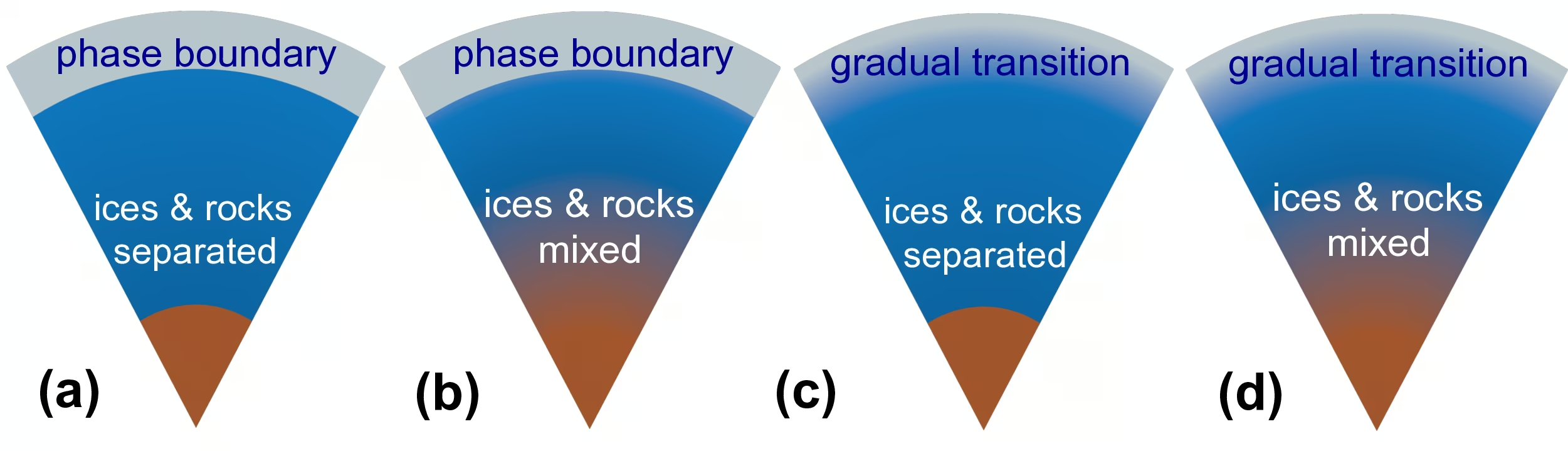
Fig. 11.37 Schematic possible internal structures of an ice giant from Helled et al. [2020]. Panels (a) through (d) illustrate increasingly gradual compositional transitions: (a) sharp boundaries between H/He envelope, ices, and rock; (b) sharp envelope/ice boundary but a gradual ice/rock transition; (c) gradual envelope/ice transition with a sharp ice/rock boundary; (d) fully gradual transitions from envelope through ice to rock with a global composition gradient. The Voyager-era gravity data alone cannot distinguish among these possibilities, which is one of the central motivations for a dedicated ice giant orbiter.#
At high pressures (\(\sim 100\) to 400 GPa and several thousand kelvins), water enters a superionic state where oxygen forms a rigid lattice while protons diffuse as a fluid [Millot et al., 2019]; a convecting shell of ionic fluid water above this stably stratified superionic layer sustains a dynamo without metallic hydrogen [Soderlund and Stanley, 2020].
Unlike dipole-dominated Jupiter and Saturn, Uranus and Neptune have multipolar magnetic fields. At Uranus, the dipole is tilted \(\sim 59^\circ\) and offset by one-third of the planetary radius [Stone and Miner, 1986]. At Neptune, the dipole is tilted \(\sim 47^\circ\) and offset by roughly half a planetary radius [Connerney et al., 1991]. This geometry indicates that the dynamo operates in a thin outer shell of conducting fluid rather than a deep core.
11.4.4. Triton#
Triton, the largest moon of Neptune, is a captured Kuiper Belt object. It is the only large moon in the solar system in a retrograde orbit (orbiting opposite to planetary rotation), inclined at \(\sim 157^\circ\). Early capture likely occurred through binary disruption during a close pass to Neptune [Agnor and Hamilton, 2006].
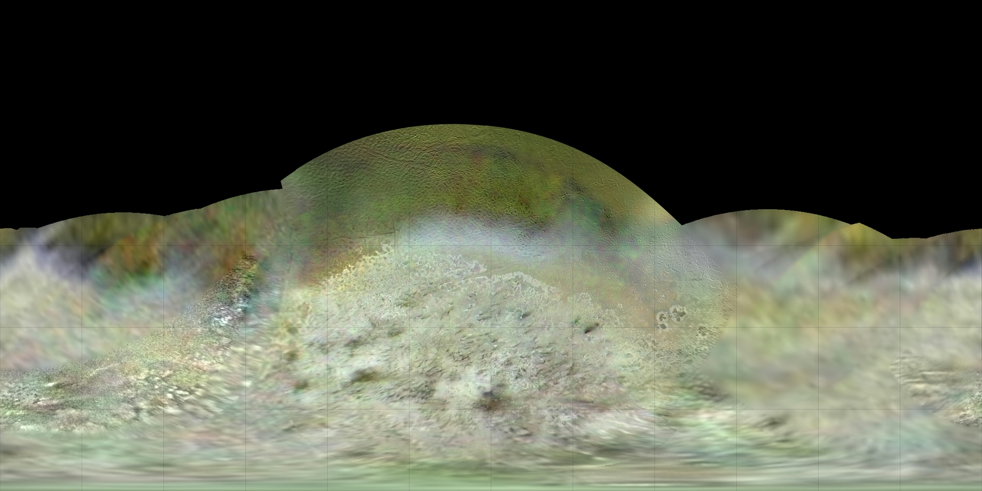
Fig. 11.38 Triton’s southern hemisphere as imaged by Voyager 2 in August 1989. Image credit: NASA/JPL-Caltech.#
Crater counts indicate a maximum surface age of about 100 Myr (Fig. 11.38). Voyager 2 observed 8 km tall dark plumes near the south pole, interpreted as nitrogen geysers driven by solar sublimation of \(\mathrm{N_2}\) ice [Smith et al., 1989]. Beside Io and Enceladus, Triton is the only outer solar system body known to host active surface eruptions. A tenuous \(\sim 14\) microbar nitrogen atmosphere supports an active cycle between ice and atmosphere.
Post-capture tidal heating damped Triton’s eccentricity within a few hundred Myr, possibly melting the interior to produce a subsurface water and ammonia ocean [McKinnon et al., 1995]. Triton shares compositional ancestry with Pluto (Lecture 12).
11.4.5. Ice giant rings#
Both Uranus and Neptune have ring systems that are much fainter and darker than Saturn’s. The first nine Uranian rings were discovered in 1977 from stellar occultations, the dimming of a star passing behind the planet; thirteen narrow rings (\(\lesssim\)10 km wide) are known today. The prominent epsilon ring at \(\sim\)51,000 km is confined by shepherd moonlets, small moons that gravitationally constrain ring edges.
Neptune’s rings were first detected as discontinuous arcs during stellar occultations. Voyager 2 showed that the outermost Adams ring contains five bright arcs trapped by resonances with Galatea (Fig. 11.39).
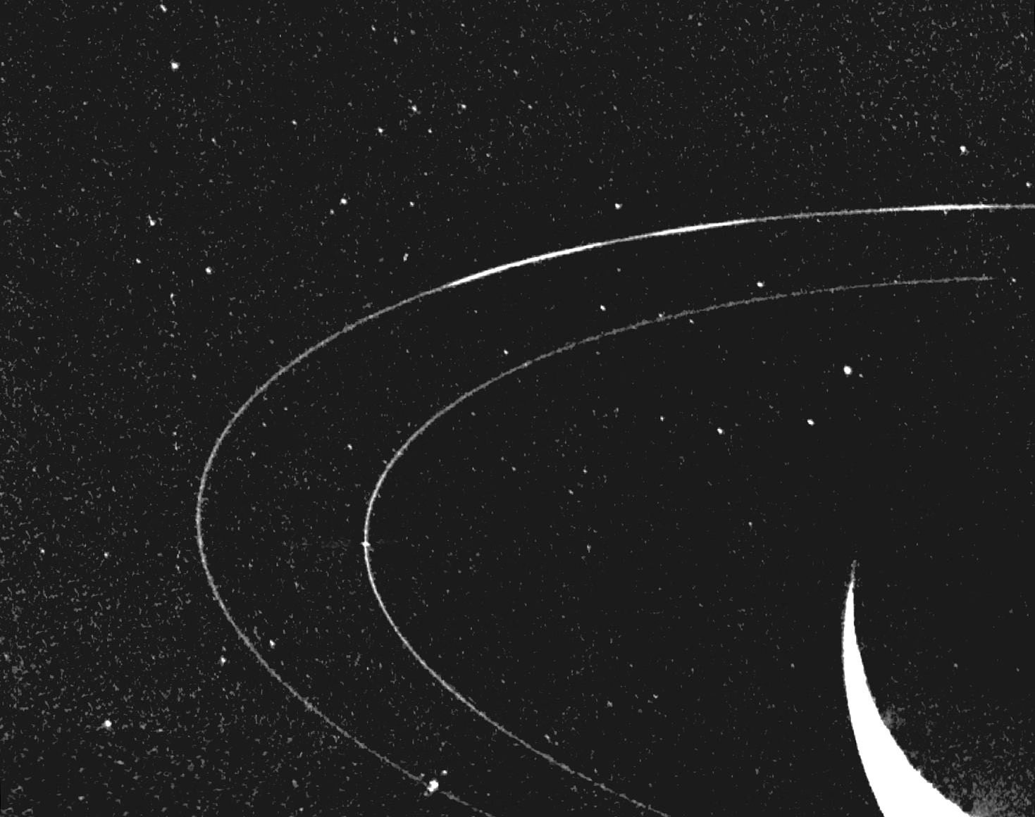
Fig. 11.39 Backscattered-light view of Neptune’s rings from Voyager 2 in 1989. The two brightest features are the Adams ring (outer) and the Le Verrier ring (inner). The arcs in the Adams ring are gravitationally trapped at specific longitudes by resonances with the inner moon Galatea. Image credit: NASA/JPL-Caltech.#
Fig. 11.40 shows the full ring system in forward-scattered light.
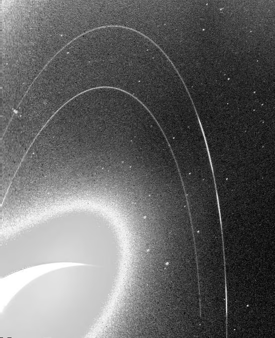
Fig. 11.40 Long-exposure forward-scattered view of Neptune’s rings showing the full ring system, including the arcs in the Adams ring and the diffuse material between the named rings. Image credit: NASA/JPL-Caltech.#
Both ice giant ring systems are dominated by dark, carbon-rich material rather than Saturn’s water ice. This compositional difference suggests that ice giant rings form from the disruption of small inner moons. In 2023, JWST observations resolved fine ring structure at Uranus [de Pater et al., 2022] and imaged Neptune’s Adams arcs and Le Verrier ring.
11.5. Part 3: Comparative payoff and exploration frontier#
11.5.1. Why gas giants and ice giants diverged#
In core accretion (Lecture 2), giant planets begin as solid cores that accrete gas from the protoplanetary disk. When a core reaches a critical mass (\(\sim\)10 \(\Mearth\)), the attracted gas contracts dynamically and triggers runaway gas accretion to capture a massive \(\mathrm{H_2}\)/He envelope. Because disk lifetimes are only \(\sim\)3 to 5 Myr, envelope growth must occur before the gas disperses (Fig. 11.41).
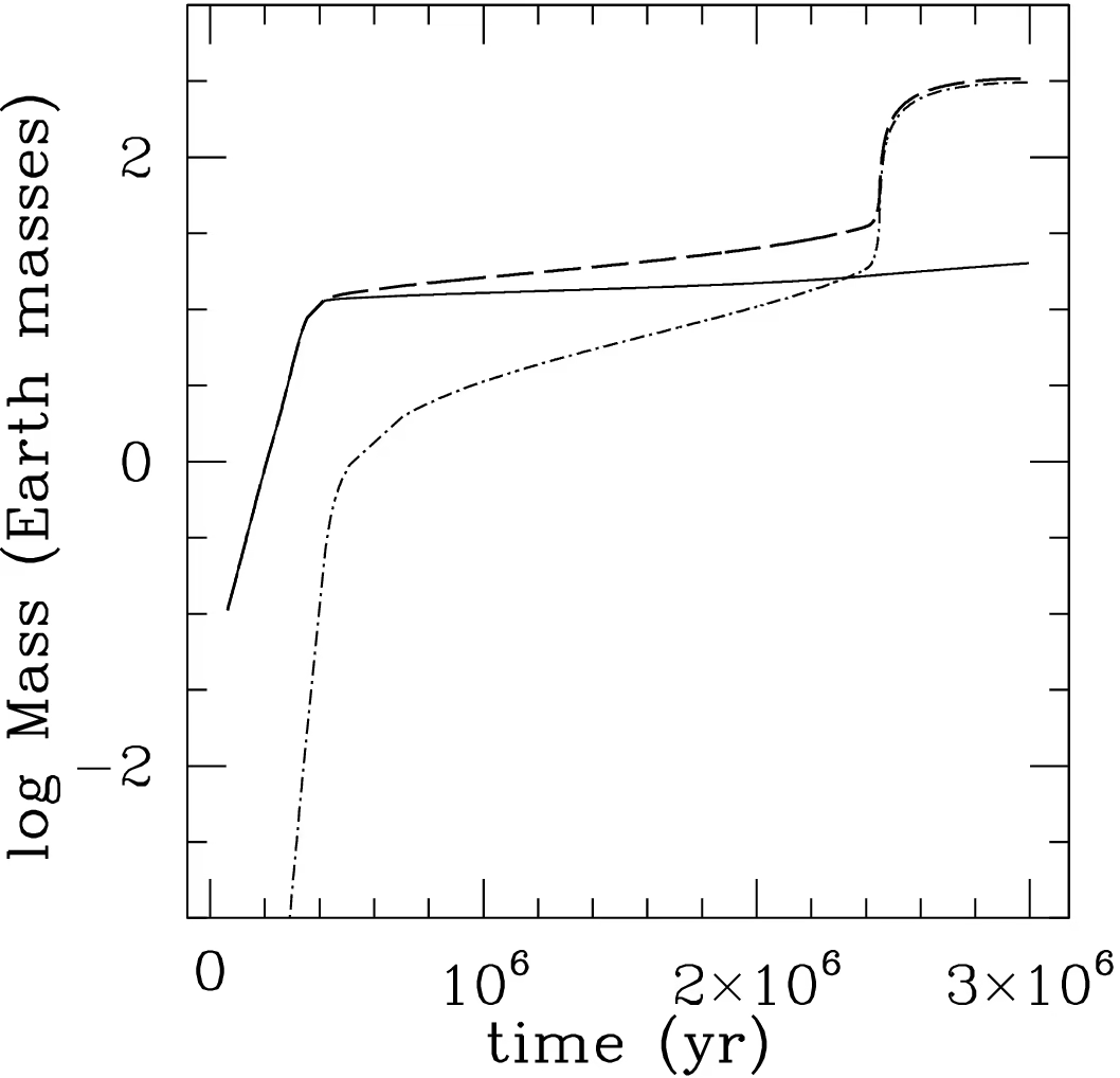
Fig. 11.41 Giant planet mass evolution via core accretion at 5.2 AU (Helled et al. [2014], based on simulations from Lissauer et al. [2009]). The curves trace core mass (solid), envelope mass (dash-dotted), and total mass (dashed) through rapid initial core assembly, quasi-hydrostatic envelope contraction, and runaway gas accretion once envelope mass exceeds core mass. Reproduced from Helled et al. [2014].#
Jupiter and Saturn reached the critical mass early. They captured massive envelopes before disk dispersal. Uranus and Neptune reached critical mass too late or formed where gas surface density was low, capturing only a few Earth masses of gas. Under the Nice model of post-formation orbital migration (Lecture 2; [Nesvorný, 2018, Tsiganis et al., 2005]), the ice giants migrated late and scattered trans-Neptunian planetesimals after disk dispersal. Their 10 to 20 \(\Mearth\) masses therefore represent a natural intermediate outcome of core accretion in the outer solar system.
11.5.2. Common themes across all four giants#
Despite the gas/ice dichotomy, the four giants share key commonalities.
Thermal emission exceeds absorbed sunlight on Neptune (\(\sim 2.6\times\)), Saturn (\(\sim 1.8\times\), driven by helium rain), and Jupiter (\(\sim 1.7\times\), driven by Kelvin-Helmholtz contraction). Uranus is the sole exception with an anomalously low excess.
All four bodies host banded atmospheres with strong zonal jets (east-west winds). Equatorial winds blow eastward on Jupiter (\(\sim 180\) m s\(^{-1}\)) and Saturn (\(\sim 400\) m s\(^{-1}\)), but westward on Neptune (\(\sim 400\) m s\(^{-1}\)) and Uranus (\(\sim 50\) to \(100\) m s\(^{-1}\)).
Electrically conducting fluid interiors generate global magnetic fields on all four planets. The dynamo source is metallic hydrogen in Jupiter and Saturn, but ionic fluid in Uranus and Neptune. Gas giants produce dipole-dominated fields, whereas ice giants exhibit multipolar, off-axis fields (Fig. 11.42).
Moon and ring systems record each giant’s dynamical history. Jupiter hosts the four Galilean moons and a faint dust ring; Saturn possesses the A through F rings, dozens of icy moons, and Titan. Uranus has narrow rings and five mid-sized moons, while Neptune has ring arcs and the captured Triton.
The four giants are laboratories for exoplanet populations. As shown in Lecture 13, the most common exoplanets are sub-Neptunes and Neptunes (\(\sim 2\) to \(4\,\Rearth\)) alongside hot Jupiters (\(\sim 1\,\Rjup\)). Our giant planets provide the only spatially resolved ground truth for these systems.
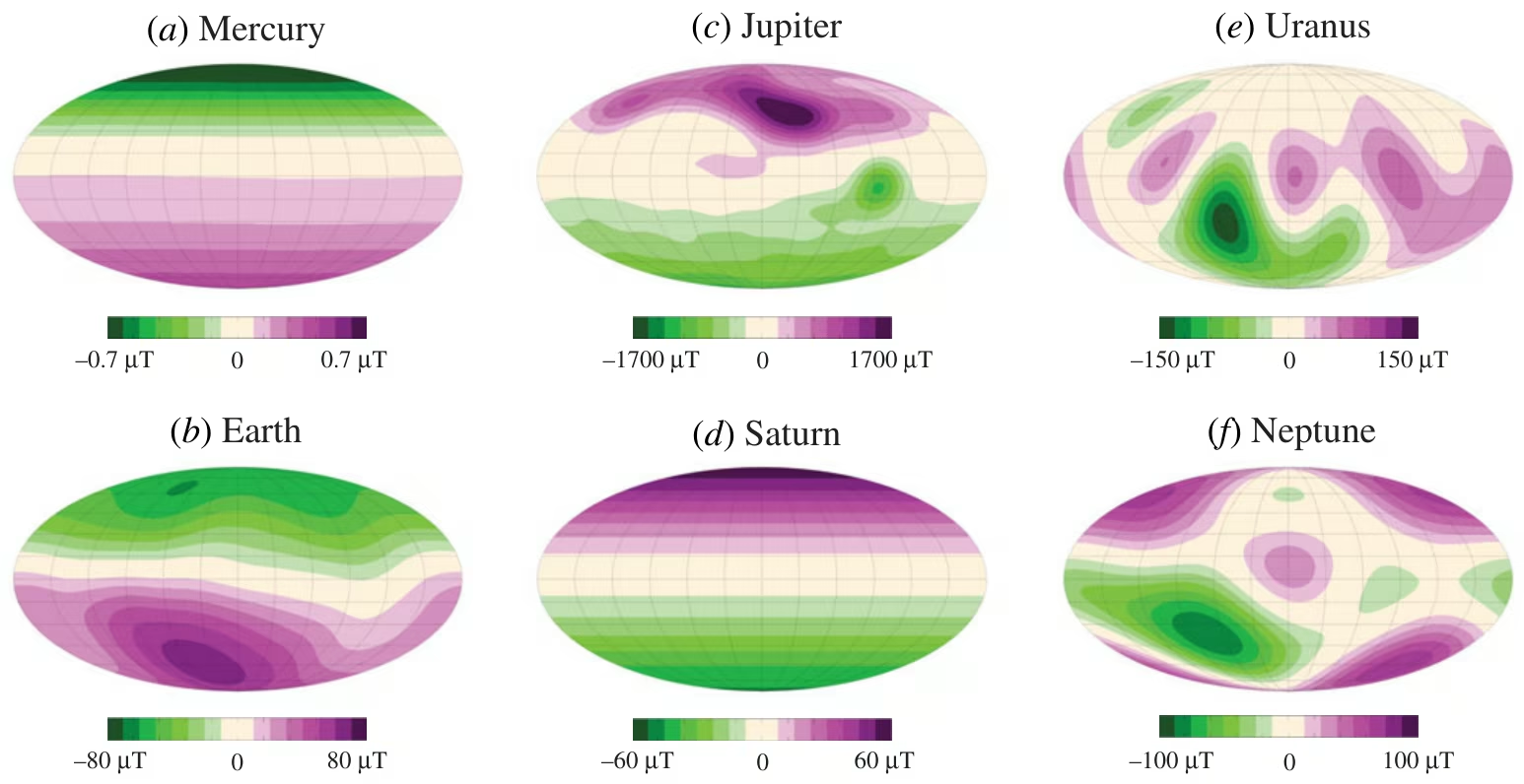
Fig. 11.42 Radial magnetic field at the surface of (a) Mercury, (b) Earth, (c) Jupiter, (d) Saturn, (e) Uranus and (f) Neptune in Mollweide projection, the panels ordered column-wise and each with its own colour scale. Jupiter and Saturn carry dipoles nearly aligned with the rotation axis; the Uranus and Neptune fields are multipolar, tilted and offset from the planetary centre. Reproduced from Soderlund and Stanley [2020], Fig. 1.#
11.5.3. What we still don’t know#
Major open questions include:
How are heavy elements partitioned between rock, ice, and gas inside Uranus and Neptune?
What sustains Neptune’s strong internal heat flow compared to Uranus?
When did Saturn’s rings form, and how long will they persist?
Are the chemistry in Enceladus’s plumes and on Titan compatible with life?
These questions require new in-situ probes or dedicated orbiters.
11.5.4. JUICE vs Europa Clipper: two ocean-world missions#
In the early 2030s, two complementary missions will arrive at Jupiter to explore the icy Galilean moons. NASA’s Europa Clipper is dedicated to Europa, performing \(\sim\)50 close flybys from Jovian orbit to characterise the ice shell, subsurface ocean, and active plumes (Fig. 11.43; Lecture 8).
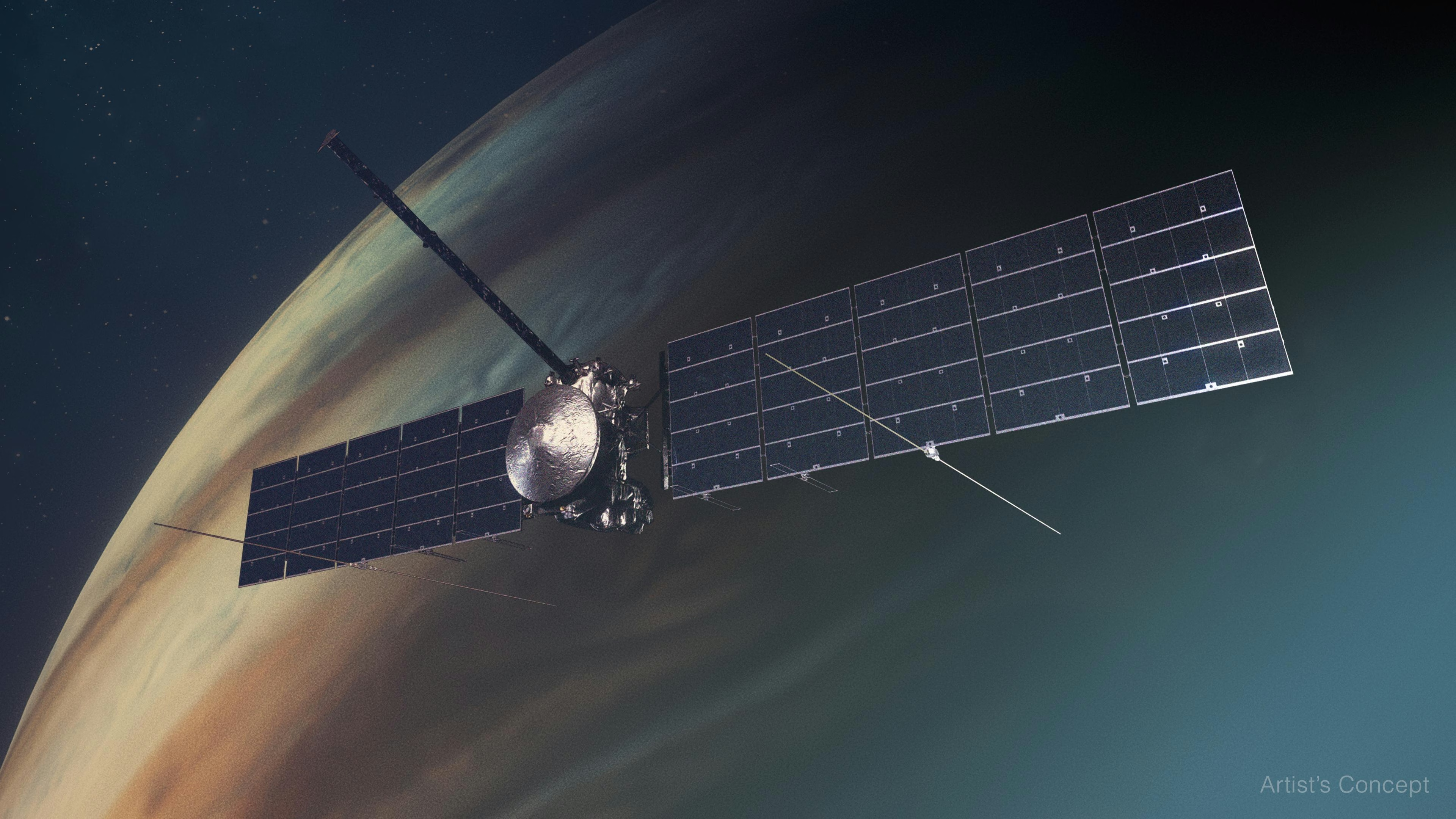
Fig. 11.43 Artist’s concept of NASA’s Europa Clipper approaching Jupiter, whose cloud bands fill the background. Clipper launched in October 2024, will arrive at Jupiter in 2030, and will conduct \(\sim\)50 close flybys of Europa from a Jovian orbit while sampling any plumes, mapping the ice shell, and constraining the ocean. Image credit: NASA/JPL-Caltech.#
ESA’s JUICE characterises the broader Jovian satellite system, performing multiple flybys of Europa, Callisto, and Ganymede before entering orbit around Ganymede in 2034. Operating simultaneously in the Jovian system during the mid-2030s enables cross-calibration of magnetic and plasma measurements across the icy Galilean moons.
11.5.5. The Voyager legacy#
The lesson of Voyager is twofold. First, the scientific return from a flyby (a single short visit) is finite and cannot substitute for sustained investigation. Ice giant knowledge is 35 years out of date. Gas giant knowledge, by contrast, has been continuously refreshed by Galileo, Cassini, Juno, and JWST, whereas Voyager 2 remains the only mission to have visited the ice giants.
Second, data from a well-designed mission continue to yield new science when combined with new theoretical tools and laboratory experiments. A single mission to the ice giants in the 2030s could anchor science for the rest of the twenty-first century. Fig. 11.44 traces the Grand Tour that gave us those single visits: one spacecraft and four gravity assists during a rare planetary alignment.
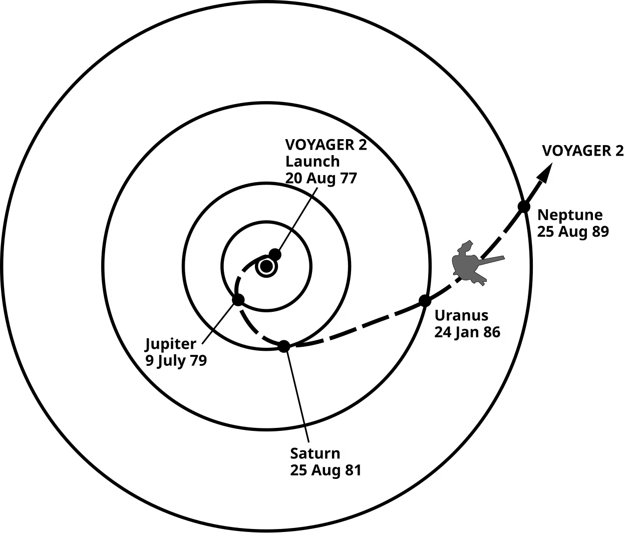
Fig. 11.44 Trajectory of NASA’s Voyager 2 spacecraft during its grand tour of the outer solar system. Successive gravity assists at Jupiter (1979), Saturn (1981), Uranus (1986), and Neptune (1989) allowed a single spacecraft to visit all four giant planets during a rare planetary alignment. Credit: NASA/JPL, public domain.#
11.5.6. Future ice giant missions#
The 2022 US Planetary Science Decadal Survey identified a Uranus orbiter and probe (a mission combining an orbiter and atmospheric entry probe) as the highest-priority flagship mission for the 2030s [National Academies of Sciences, Engineering, and Medicine, 2022]. Launch in the early 2030s with a Jupiter gravity assist would reach Uranus in the late 2030s or early 2040s to measure deep noble gas, isotopic, and molecular composition.
11.6. Summary and takeaways#
Gas giants and ice giants form a compositional continuum, from the H/He-dominated Jupiter and Saturn to the ice-dominated Uranus and Neptune; the sequence records the timing of core formation, the available disk gas, and the migration history.
Both gas giants now appear to host extended, dilute heavy-element distributions rather than compact cores, a major reinterpretation driven by Juno (Jupiter) and Cassini Grand Finale + ring seismology (Saturn).
Saturn’s rings are young and transient, with current best estimates of \(\sim\)100 Myr age and a comparable remaining lifetime.
The Galilean moons span a remarkable diversity: tidally heated and volcanic Io, ocean-bearing Europa, dynamo-generating Ganymede, and ancient, partially differentiated Callisto, alongside ocean worlds Titan, Enceladus, and Triton.
The ice giants are the most under-explored planets in the solar system; everything known in detail about Uranus and Neptune comes from single 1980s flybys, making a dedicated orbiter overdue.
The Roche limit explains why rings exist where they do and why small bodies cannot coalesce close to their host planet, predicting the outer edge of Saturn’s A ring to within \(\sim\)10%.
The exploration frontier is extraordinary: Juno, JUICE, Europa Clipper, and a future Uranus orbiter will collectively transform outer solar system science between now and 2045.
11.7. References#
Adriani, A., Mura, A., Orton, G., Hansen, C., Altieri, F., Moriconi, M. L., Rogers, J., Eichstädt, G., Momary, T., Ingersoll, A. P., Filacchione, G., Sindoni, G., Tabataba-Vakili, F., Dinelli, B. M., Fabiano, F., Bolton, S. J., Connerney, J. E. P., Atreya, S. K., Lunine, J. I., Tosi, F., Migliorini, A., Grassi, D., Piccioni, G., Noschese, R., Cicchetti, A., Plainaki, C., Olivieri, A., O'Neill, M. E., Turrini, D., Stefani, S., Sordini, R., and Amoroso, M. 2018. “Clusters of cyclones encircling Jupiter's poles.” Nature, 555:216–219. doi:10.1038/nature25491, https://ui.adsabs.harvard.edu/abs/2018Natur.555..216A/abstract.
Agnor, C. B. and Hamilton, D. P. 2006. “Neptune's capture of its moon Triton in a binary–planet gravitational encounter.” Nature, 441:192–194. doi:10.1038/nature04792, https://ui.adsabs.harvard.edu/abs/2006Natur.441..192A/abstract.
Anderson, J. D., Jacobson, R. A., McElrath, T. P., Moore, W. B., Schubert, G., and Thomas, P. C. 2001. “Shape, mean radius, gravity field, and interior structure of Callisto.” Icarus, 153(1):157–161. doi:10.1006/icar.2001.6664, https://ui.adsabs.harvard.edu/abs/2001Icar..153..157A/abstract.
Charnoz, S., Morbidelli, A., Dones, L., and Salmon, J. 2009. “Did Saturn's rings form during the Late Heavy Bombardment?.” Icarus, 199(2):413–428. doi:10.1016/j.icarus.2008.10.019, https://ui.adsabs.harvard.edu/abs/2009Icar..199..413C/abstract.
Connerney, J. E. P., Acuña, M. H., and Ness, N. F. 1991. “The magnetic field of Neptune.” Journal of Geophysical Research, 96:19023–19042. doi:10.1029/91JA01165, https://ui.adsabs.harvard.edu/abs/1991JGR....9619023C/abstract.
Connerney, J. E. P., Timmins, S., Oliversen, R. J., Espley, J. R., Joergensen, J. L., Kotsiaros, S., Joergensen, P. S., Merayo, J. M. G., Herceg, M., Bloxham, J., Moore, K. M., Bolton, S. J., and Levin, S. M. 2022. “A new model of Jupiter's magnetic field at the completion of Juno's prime mission.” Journal of Geophysical Research: Planets, 127(2):e2021JE007055. doi:10.1029/2021JE007055, https://ui.adsabs.harvard.edu/abs/2022JGRE..12707055C/abstract.
Crida, A., Charnoz, S., Hsu, H.-W., and Dones, L. 2019. “Are Saturn's rings actually young?.” Nature Astronomy, 3:967–970. doi:10.1038/s41550-019-0876-y, https://ui.adsabs.harvard.edu/abs/2019NatAs...3..967C/abstract.
de Pater, I., Molter, E. M., Hammel, H. B., Tollefson, J. W., Wong, M. H., Roman, M. T., Carter, S., Rivkin, A., Verbiscer, A., Hueso, R., Fletcher, L. N., Stallard, T., Hofstadter, M., Sromovsky, L., Fry, P., Tiscareno, M., Norwood, J., and Strange, N. 2022. “JWST observations of the Uranian system: inner satellites and the rings.” The Astronomical Journal, 164:269. doi:10.3847/1538-3881/ac9aab, https://ui.adsabs.harvard.edu/abs/2022AJ....164..269D/abstract.
de Pater, Imke and Lissauer, Jack J. 2010. Planetary Sciences. Cambridge University Press, Cambridge, 2nd edition. doi:10.1017/cbo9780511780561.
Fortney, Jonathan J. and Nettelmann, Nadine. 2010. “The interior structure, composition, and evolution of giant planets.” Space Science Reviews, 152(1–4):423–447. doi:10.1007/s11214-009-9582-x, arXiv:0912.0533, https://ui.adsabs.harvard.edu/abs/2010SSRv..152..423F/abstract.
Grasset, O., Dougherty, M. K., Coustenis, A., Bunce, E. J., Erd, C., Titov, D., Blanc, M., Coates, A., Drossart, P., Fletcher, L. N., Hussmann, H., Jaumann, R., Krupp, N., Lebreton, J.-P., Prieto-Ballesteros, O., Tortora, P., Tosi, F., and Van Hoolst, T. 2013. “JUpiter ICy moons Explorer (JUICE): an ESA mission to orbit Ganymede and to characterise the Jupiter system.” Planetary and Space Science, 78:1–21. doi:10.1016/j.pss.2012.12.002, https://ui.adsabs.harvard.edu/abs/2013P&SS...78....1G/abstract.
Helled, R., Nettelmann, N., and Guillot, T. 2020. “Uranus and neptune: origin, evolution and internal structure.” Space Science Reviews, 216:38. doi:10.1007/s11214-020-00660-3, https://ui.adsabs.harvard.edu/abs/2020SSRv..216...38H/abstract.
Helled, Ravit, Bodenheimer, Peter, Podolak, Morris, Boley, Aaron, Meru, Farzana, Nayakshin, Sergei, Fortney, Jonathan J., Mayer, Lucio, Alibert, Yann, and Boss, Alan P. 2014. “Giant planet formation, evolution, and internal structure.” In Beuther, Henrik, Klessen, Ralf S., Dullemond, Cornelis P., and Henning, Thomas, editors, Protostars and Planets VI, pages 643–665. University of Arizona Press. doi:10.2458/azu_uapress_9780816531240-ch028, arXiv:1311.1142, https://ui.adsabs.harvard.edu/abs/2014prpl.conf..643H/abstract.
Howell, Samuel M. and Pappalardo, Robert T. 2020. “NASA's Europa Clipper: a mission to a potentially habitable ocean world.” Nature Communications, 11:1311. doi:10.1038/s41467-020-15160-9, https://ui.adsabs.harvard.edu/abs/2020NatCo..11.1311H/abstract.
Iess, L., Folkner, W. M., Durante, D., Parisi, M., Kaspi, Y., Galanti, E., Guillot, T., Hubbard, W. B., Stevenson, D. J., Anderson, J. D., Buccino, D. R., Casajus, L. Gomez, Milani, A., Park, R., Racioppa, P., Serra, D., Tortora, P., Zannoni, M., Cao, H., Helled, R., Lunine, J. I., Miguel, Y., Militzer, B., Wahl, S., Connerney, J. E. P., Levin, S. M., and Bolton, S. J. 2018. “Measurement of Jupiter's asymmetric gravity field.” Nature, 555:220–222. doi:10.1038/nature25776, https://ui.adsabs.harvard.edu/abs/2018Natur.555..220I/abstract.
Iess, L., Jacobson, R. A., Ducci, M., Stevenson, D. J., Lunine, J. I., Armstrong, J. W., Asmar, S. W., Racioppa, P., Rappaport, N. J., and Tortora, P. 2012. “The tides of Titan.” Science, 337(6093):457–459. doi:10.1126/science.1219631, https://ui.adsabs.harvard.edu/abs/2012Sci...337..457I/abstract.
Iess, L., Militzer, B., Kaspi, Y., Nicholson, P., Durante, D., Racioppa, P., Anabtawi, A., Galanti, E., Hubbard, W., Mariani, M. J., Tortora, P., Wahl, S., and Zannoni, M. 2019. “Measurement and implications of Saturn's gravity field and ring mass.” Science, 364(6445):eaat2965. doi:10.1126/science.aat2965, https://ui.adsabs.harvard.edu/abs/2019Sci...364.2965I/abstract.
Kaspi, Y., Galanti, E., Hubbard, W. B., Stevenson, D. J., Bolton, S. J., Iess, L., Guillot, T., Bloxham, J., Connerney, J. E. P., Cao, H., Durante, D., Folkner, W. M., Helled, R., Ingersoll, A. P., Levin, S. M., Lunine, J. I., Miguel, Y., Militzer, B., Parisi, M., and Wahl, S. M. 2018. “Jupiter's atmospheric jet streams extend thousands of kilometres deep.” Nature, 555:223–226. doi:10.1038/nature25793, https://ui.adsabs.harvard.edu/abs/2018Natur.555..223K/abstract.
Kegerreis, J. A., Teodoro, L. F. A., Eke, V. R., Massey, R. J., Catling, D. C., Fryer, C. L., Korycansky, D. G., Warren, M. S., and Zahnle, K. J. 2018. “Consequences of giant impacts on early Uranus for rotation, internal structure, debris, and atmospheric erosion.” The Astrophysical Journal, 861(1):52. doi:10.3847/1538-4357/aac725, arXiv:1803.07083, https://ui.adsabs.harvard.edu/abs/2018ApJ...861...52K/abstract.
Khurana, K. K., Kivelson, M. G., Stevenson, D. J., Schubert, G., Russell, C. T., Walker, R. J., and Polanskey, C. 1998. “Induced magnetic fields as evidence for subsurface oceans in Europa and Callisto.” Nature, 395:777–780. doi:10.1038/27394, https://ui.adsabs.harvard.edu/abs/1998Natur.395..777K/abstract.
Lissauer, Jack J., Hubickyj, Olenka, D'Angelo, Gennaro, and Bodenheimer, Peter. 2009. “Models of Jupiter's growth incorporating thermal and hydrodynamic constraints.” Icarus, 199(2):338–350. doi:10.1016/j.icarus.2008.10.004, arXiv:0810.5186, https://ui.adsabs.harvard.edu/abs/2009Icar..199..338L/abstract.
Lorenz, R. D., Turtle, E. P., Barnes, J. W., Trainer, M. G., Adams, D. S., Hibbard, K. E., Sheldon, C. Z., Zacny, K., Peplowski, P. N., Lawrence, D. J., Ravine, M. A., McGee, T. G., Sotzen, K. S., MacKenzie, S. M., Langelaan, J. W., Schmitz, S., Wolfarth, L. S., and Bedini, P. D. 2018. “Dragonfly: a rotorcraft lander concept for scientific exploration at Titan.” Johns Hopkins APL Technical Digest, 34(3):374–387. https://ui.adsabs.harvard.edu/abs/2018JHATD..34..374L/abstract.
Mankovich, Christopher, Marley, Mark S., Fortney, Jonathan J., and Movshovitz, Naor. 2019. “Cassini ring seismology as a probe of Saturn's interior. I. rigid rotation.” The Astrophysical Journal, 871(1):1. doi:10.3847/1538-4357/aaf798, arXiv:1805.10286, https://ui.adsabs.harvard.edu/abs/2019ApJ...871....1M/abstract.
Mankovich, Christopher R. and Fuller, Jim. 2021. “A diffuse core in Saturn revealed by ring seismology.” Nature Astronomy, 5:1103–1109. doi:10.1038/s41550-021-01448-3, arXiv:2104.13385, https://ui.adsabs.harvard.edu/abs/2021NatAs...5.1103M/abstract.
McKinnon, W. B., Lunine, J. I., and Banfield, D. 1995. “Origin and evolution of Triton.” Neptune and Triton (D. P. Cruikshank, ed.), pages 807–877. https://ui.adsabs.harvard.edu/abs/1995netr.conf..807M/abstract.
Militzer, B., Hubbard, W. B., Wahl, S., Lunine, J. I., Galanti, E., Kaspi, Y., Miguel, Y., Guillot, T., Moore, K. M., Parisi, M., Connerney, J. E. P., Helled, R., Cao, H., Mankovich, C., Stevenson, D. J., Park, R. S., Wong, M., Atreya, S. K., Anderson, J., and Bolton, S. J. 2022. “Juno spacecraft measurements of Jupiter's gravity imply a dilute core.” The Planetary Science Journal, 3(8):185. doi:10.3847/PSJ/ac7ec8, https://ui.adsabs.harvard.edu/abs/2022PSJ.....3..185M/abstract.
Millot, M., Coppari, F., Rygg, J. R., Correa Barrios, A., Hamel, S., Swift, D. C., and Eggert, J. H. 2019. “Nanosecond x-ray diffraction of shock-compressed superionic water ice.” Nature, 569:251–255. doi:10.1038/s41586-019-1114-6, https://ui.adsabs.harvard.edu/abs/2019Natur.569..251M/abstract.
Morbidelli, A., Tsiganis, K., Batygin, K., Crida, A., and Gomes, R. 2012. “Explaining why the Uranian satellites have equatorial prograde orbits despite the large planetary obliquity.” Icarus, 219(2):737–740. doi:10.1016/j.icarus.2012.03.025, arXiv:1208.4685, https://ui.adsabs.harvard.edu/abs/2012Icar..219..737M/abstract.
Nesvorný, David. 2018. “Dynamical evolution of the early solar system.” Annual Review of Astronomy and Astrophysics, 56:137–174. doi:10.1146/annurev-astro-081817-052028, arXiv:1807.06647, https://ui.adsabs.harvard.edu/abs/2018ARA%26A..56..137N/abstract.
Niemann, H. B., Atreya, S. K., Carignan, G. R., Donahue, T. M., Haberman, J. A., Harpold, D. N., Hartle, R. E., Hunten, D. M., Kasprzak, W. T., Mahaffy, P. R., Owen, T. C., and Way, S. H. 1998. “The composition of the Jovian atmosphere as determined by the Galileo probe mass spectrometer.” Journal of Geophysical Research: Planets, 103(E10):22831–22845. doi:10.1029/98JE01050, https://ui.adsabs.harvard.edu/abs/1998JGR...10322831N/abstract.
O'Donoghue, J., Moore, L., Connerney, J., Melin, H., Stallard, T. S., Miller, S., and Baines, K. H. 2019. “Observations of the chemical and thermal response of `ring rain' on Saturn's ionosphere.” Icarus, 322:251–260. doi:10.1016/j.icarus.2018.10.027, https://ui.adsabs.harvard.edu/abs/2019Icar..322..251O/abstract.
Pappalardo, R. T., Belton, M. J. S., Breneman, H. H., Carr, M. H., Chapman, C. R., Collins, G. C., Denk, T., Fagents, S., Geissler, P. E., Giese, B., Greeley, R., Greenberg, R., Head, J. W., Helfenstein, P., Hoppa, G., Kadel, S. D., Klaasen, K. P., Klemaszewski, J. E., Magee, K., McEwen, A. S., Moore, J. M., Moore, W. B., Neukum, G., Phillips, C. B., Prockter, L. M., Schubert, G., Senske, D. A., Sullivan, R. J., Thomas, P. C., Turtle, E. P., Wagner, R., and Williams, K. K. 1999. “Does Europa have a subsurface ocean? evaluation of the geological evidence.” Journal of Geophysical Research: Planets, 104(E10):24015–24055. doi:10.1029/1998JE000628, https://ui.adsabs.harvard.edu/abs/1999JGR...10424015P/abstract.
Park, R. S., Jacobson, R. A., Gomez Casajus, L., Nimmo, F., Ermakov, A. I., Keane, J. T., McEwen, A. S., Steinbrügge, G., Akiba, R., Bills, B. G., Buccino, D. R., Idini, B., Magnanini, A., Mazarico, E., Parisi, M., Mura, A., Durante, D., Tortora, P., Zannoni, M., Anderson, J. D., Connerney, J. E. P., Levin, S. M., and Bolton, S. J. 2025. “Io's tidal response precludes a shallow magma ocean.” Nature, 638:69–73. doi:10.1038/s41586-024-08442-5, https://ui.adsabs.harvard.edu/abs/2025Natur.638...69P/abstract.
Peale, Stanton J., Cassen, Patrick, and Reynolds, Ray T. 1979. “Melting of Io by tidal dissipation.” Science, 203(4383):892–894. doi:10.1126/science.203.4383.892, https://ui.adsabs.harvard.edu/abs/1979Sci...203..892P/abstract.
Pearl, J. C. and Conrath, B. J. 1991. “The albedo, effective temperature, and energy balance of Neptune, as determined from Voyager data.” Journal of Geophysical Research, 96:18921–18930. doi:10.1029/91JA01087, https://ui.adsabs.harvard.edu/abs/1991JGR....9618921P/abstract.
Pearl, J. C., Conrath, B. J., Hanel, R. A., Pirraglia, J. A., and Coustenis, A. 1990. “The albedo, effective temperature, and energy balance of Uranus, as determined from Voyager IRIS data.” Icarus, 84:12–28. doi:10.1016/0019-1035(90)90155-3, https://ui.adsabs.harvard.edu/abs/1990Icar...84...12P/abstract.
Porco, C. C., Helfenstein, P., Thomas, P. C., Ingersoll, A. P., Wisdom, J., West, R., Neukum, G., Denk, T., Wagner, R., Roatsch, T., Kieffer, S., Turtle, E., McEwen, A., Johnson, T. V., Rathbun, J., Veverka, J., Wilson, D., Perry, J., Spitale, J., Brahic, A., Burns, J. A., DelGenio, A. D., Dones, L., Murray, C. D., and Squyres, S. 2006. “Cassini observes the active south pole of Enceladus.” Science, 311(5766):1393–1401. doi:10.1126/science.1123013, https://ui.adsabs.harvard.edu/abs/2006Sci...311.1393P/abstract.
Postberg, F., Sekine, Y., Klenner, F., Glein, C. R., Zou, Z., Abel, B., Furuya, K., Hillier, J. K., Khawaja, N., Kempf, S., Noelle, L., Saito, T., Schmidt, J., Shibuya, T., Srama, R., and Tan, S. 2023. “Detection of phosphates originating from Enceladus's ocean.” Nature, 618:489–493. doi:10.1038/s41586-023-05987-9, https://ui.adsabs.harvard.edu/abs/2023Natur.618..489P/abstract.
Roche, Édouard. 1849. “La figure d'une masse fluide soumise à l'attraction d'un point éloigné.” Académie des Sciences de Montpellier: Mémoires de la section des sciences, 1:243–262. Classical reference for the Roche limit derivation.
Saur, J., Duling, S., Roth, L., Jia, X., Strobel, D. F., Feldman, P. D., Christensen, U. R., Retherford, K. D., McGrath, M. A., Musacchio, F., Wennmacher, A., Neubauer, F. M., Simon, S., and Hartkorn, O. 2015. “The search for a subsurface ocean in Ganymede with Hubble Space Telescope observations of its auroral ovals.” Journal of Geophysical Research: Space Physics, 120(3):1715–1737. doi:10.1002/2014JA020778, https://ui.adsabs.harvard.edu/abs/2015JGRA..120.1715S/abstract.
Smith, B. A., Soderblom, L. A., Banfield, D., Barnet, C., Basilevsky, A. T., Beebe, R. F., Bollinger, K., Boyce, J. M., Brahic, A., Briggs, G. A., Brown, R. H., Chyba, C., Collins, S. A., Colvin, T., Cook, A. F., Crisp, D., Croft, S. K., Cruikshank, D., Cuzzi, J. N., Danielson, G. E., Davies, M. E., De Jong, E., Dones, L., Godfrey, D., Goguen, J., Grenier, I., Haemmerle, V. R., Hammel, H., Hansen, C. J., Helfenstein, C. P., Howell, C., Hunt, G. E., Ingersoll, A. P., Johnson, T. V., Kargel, J., Kirk, R., Kuehn, D. I., Limaye, S., Masursky, H., McEwen, A., Morrison, D., Owen, T., Owen, W., Pollack, J. B., Porco, C. C., Rages, K., Rogers, P., Rudy, D., Sagan, C., Schwartz, J., Shoemaker, E. M., Showalter, M., Sicardy, B., Simonelli, D., Spencer, J., Sromovsky, L. A., Stoker, C., Strom, R. G., Suomi, V. E., Synnott, S. P., Terrile, R. J., Thomas, P., Thompson, W. R., Verbiscer, A., and Veverka, J. 1989. “Voyager 2 at Neptune: imaging science results.” Science, 246(4936):1422–1449. doi:10.1126/science.246.4936.1422, https://ui.adsabs.harvard.edu/abs/1989Sci...246.1422S/abstract.
Soderlund, K. M. and Stanley, S. 2020. “The underexplored frontier of ice giant dynamos.” Philosophical Transactions of the Royal Society A, 378:20190479. doi:10.1098/rsta.2019.0479, https://ui.adsabs.harvard.edu/abs/2020RSPTA.37890479S/abstract.
Stevenson, D. J. 1980. “Saturn's luminosity and magnetism.” Science, 208(4445):746–748. doi:10.1126/science.208.4445.746, https://ui.adsabs.harvard.edu/abs/1980Sci...208..746S/abstract.
Stevenson, D. J. 2020. “Jupiter's interior as revealed by Juno.” Annual Review of Earth and Planetary Sciences, 48:465–489. doi:10.1146/annurev-earth-081619-052855, https://ui.adsabs.harvard.edu/abs/2020AREPS..48..465S/abstract.
Stofan, E. R., Elachi, C., Lunine, J. I., Lorenz, R. D., Stiles, B., Mitchell, K. L., Ostro, S., Soderblom, L., Wood, C., Zebker, H., Wall, S., Janssen, M., Kirk, R., Lopes, R., Paganelli, F., Radebaugh, J., Wye, L., Anderson, Y., Allison, M., Boehmer, R., Callahan, P., Encrenaz, P., Flamini, E., Francescetti, G., Gim, Y., Hamilton, G., Hensley, S., Johnson, W. T. K., Kelleher, K., Muhleman, D., Paillou, P., Picardi, G., Posa, F., Roth, L., Seu, R., Shaffer, S., Vetrella, S., and West, R. 2007. “The lakes of Titan.” Nature, 445:61–64. doi:10.1038/nature05438, https://ui.adsabs.harvard.edu/abs/2007Natur.445...61S/abstract.
Stone, E. C. and Miner, E. D. 1986. “The Voyager 2 encounter with the Uranian system.” Science, 233(4759):39–43. doi:10.1126/science.233.4759.39, https://ui.adsabs.harvard.edu/abs/1986Sci...233...39S/abstract.
Stone, E. C. and Miner, E. D. 1989. “The Voyager 2 encounter with the Neptunian system.” Science, 246(4936):1417–1421. doi:10.1126/science.246.4936.1417, https://ui.adsabs.harvard.edu/abs/1989Sci...246.1417S/abstract.
Tiscareno, M. S. 2013. “Planetary rings.” Planets, Stars and Stellar Systems, Volume 3: Solar and Stellar Planetary Systems, pages 309. doi:10.1007/978-94-007-5606-9_7, https://ui.adsabs.harvard.edu/abs/2013pss3.book..309T/abstract.
Tsiganis, Kleomenis, Gomes, Rodney, Morbidelli, Alessandro, and Levison, Harold F. 2005. “Origin of the orbital architecture of the giant planets of the Solar System.” Nature, 435:459–461. doi:10.1038/nature03539, https://ui.adsabs.harvard.edu/abs/2005Natur.435..459T/abstract.
Wahl, Sean M., Hubbard, William B., Militzer, Burkhard, Guillot, Tristan, Miguel, Yamila, Movshovitz, Nadine, Kaspi, Yohai, Helled, Ravit, Reese, David, Galanti, Eli, Levin, Steve, Connerney, John E. P., and Bolton, Scott J. 2017. “Comparing Jupiter interior structure models to Juno gravity measurements and the role of a dilute core.” Geophysical Research Letters, 44(10):4649–4659. doi:10.1002/2017GL073160, arXiv:1707.01997, https://ui.adsabs.harvard.edu/abs/2017GeoRL..44.4649W/abstract.
Waite, J. H., Glein, C. R., Perryman, R. S., Teolis, B. D., Magee, B. A., Miller, G., Grimes, J., Perry, M. E., Miller, K. E., Bouquet, A., Lunine, J. I., Brockwell, T., and Bolton, S. J. 2017. “Cassini finds molecular hydrogen in the Enceladus plume: evidence for hydrothermal processes.” Science, 356(6334):155–159. doi:10.1126/science.aai8703, https://ui.adsabs.harvard.edu/abs/2017Sci...356..155W/abstract.
Waite, J. H., Perryman, R. S., Perry, M. E., Miller, K. E., Bell, J., Cravens, T. E., Glein, C. R., Grimes, J., Hedman, M., Cuzzi, J., Brockwell, T., Teolis, B., Moore, L., Mitchell, D. G., Persoon, A., Kurth, W. S., Wahlund, J.-E., Morooka, M., Hadid, L. Z., Chocron, S., Walker, J., Nagy, A., Yelle, R., Ledvina, S., Johnson, R., Tseng, W., Tucker, O. J., and Ip, W.-H. 2018. “Chemical interactions between Saturn's atmosphere and its rings.” Science, 362(6410):eaat2382. doi:10.1126/science.aat2382, https://ui.adsabs.harvard.edu/abs/2018Sci...362.2382W/abstract.
Wisdom, J., Dbouk, R., Militzer, B., Hubbard, W. B., Nimmo, F., Downey, B. G., and French, R. G. 2022. “Loss of a satellite could explain Saturn's obliquity and young rings.” Science, 377(6612):1285–1289. doi:10.1126/science.abn1234, https://ui.adsabs.harvard.edu/abs/2022Sci...377.1285W/abstract.
NASA Jet Propulsion Laboratory. 2026. Planetary physical parameters. NASA Solar System Dynamics, Caltech/JPL. Values derive from the IAU/IAG Working Group report (Archinal et al. 2018, Celestial Mechanics and Dynamical Astronomy 130:22) and current GM estimates. https://ssd.jpl.nasa.gov/planets/phys_par.html.
National Academies of Sciences, Engineering, and Medicine. 2022. Origins, worlds, and life: a decadal strategy for planetary science and astrobiology 2023–2032. doi:10.17226/26522, https://nap.nationalacademies.org/catalog/26522/origins-worlds-and-life-a-decadal-strategy-for-planetary-science.