Exoplanets, Detection Methods, Demographics & Characterisation

13. Exoplanets, Detection Methods, Demographics & Characterisation#

Learning objectives: By the end of this lecture, you will be able to describe the main exoplanet detection methods and their observational biases, interpret the period-radius diagram and its key features (radius valley, hot Neptune desert, peas-in-a-pod), apply the transit and radial velocity geometry to derive planetary mass, radius, and bulk density, and evaluate JWST-era atmospheric characterisation results and their implications for habitability and biosignatures.

13.1. Part 1: How we find exoplanets#

13.1.1. Historical context#

The first confirmed planets outside the solar system were announced in 1992 by Aleksander Wolszczan and Dale Frail around the radio pulsar PSR B1257+12 [Wolszczan and Frail, 1992]. The system contains two planets with minimum masses of about $3.4$ and $2.8\,\Mearth$ in $66$ and $98$ day orbits, plus a lunar-mass third body ($\sim 0.015\,\Mearth$) in a $25.34$ day orbit [Wolszczan, 1994, Wolszczan and Frail, 1992]. These post-supernova planets showed that planetary bodies can exist in environments far removed from the standard star and disk framework of Lecture 2.

In 1995 Michel Mayor and Didier Queloz used the ELODIE spectrograph to detect 51 Pegasi b, the first confirmed planet orbiting a main-sequence star, earning the 2019 Nobel Prize in Physics [Mayor and Queloz, 1995]. The planet has roughly half the mass of Jupiter on a 4.23-day orbit. A gas giant so close to its star contradicted standard models where gas giants form beyond the ice line during runaway accretion (the rapid intake of surrounding nebular gas by a growing core) [Pollack et al., 1996]. This discovery motivated the planetary migration interpretation, which won out over in-situ formation within a few years: planets form at large orbital distances and move inward through disk interactions (Lecture 2).

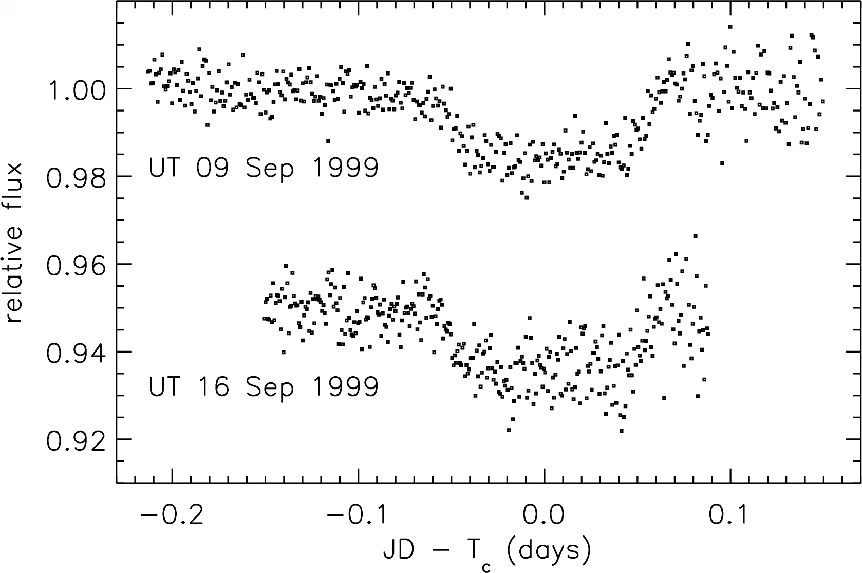
../_images/hd209458b_first_transit.avif — Fig. 13.1 The first ground-based detection of a transiting exoplanet, **HD 209458 b**, observed with the STARE photometer over two nights in September 1999. Each successive transit dropped the relative flux of the host star by approximately 1.7 per cent, exactly the depth predicted from the radial velocity mass and an inferred Jupiter-like radius. From Charbonneau *et al.* [2000]; an independent simultaneous detection was reported by Henry *et al.* [2000]. After this point exoplanets were no longer abstract Doppler signals: they were physical objects whose sizes could be measured directly.#

In 1999 the first transit detection of HD 209458 b combined transit depth and radial velocity to determine the first planetary bulk density (total mass divided by volume) (Fig. 13.1). This confirmed that hot Jupiters (Jupiter-mass planets on orbits of only a few days) are gas-dominated bodies rather than high-density objects. By 2026 the NASA Exoplanet Archive recorded more than 6000 confirmed exoplanets in more than 4500 planetary systems [NASA Exoplanet Science Institute, 2025].

13.1.2. Radial velocity method#

A planet of mass $m_p$ and host star of mass $M_\star$ orbit their common barycentre with stellar orbit radius $a_\star = (m_p / M_\star)\,a_p$, spanning about one solar radius for a Jupiter analogue and less than a thousandth of a solar radius for an Earth analogue. This stellar reflex motion causes periodic Doppler shifts in stellar absorption lines, yielding the orbital period $P$, eccentricity $e$, and semi-amplitude $K_\star$. When the star moves away from the observer, its lines shift to longer wavelengths; when it moves towards the observer, they shift to shorter wavelengths (Fig. 13.2).

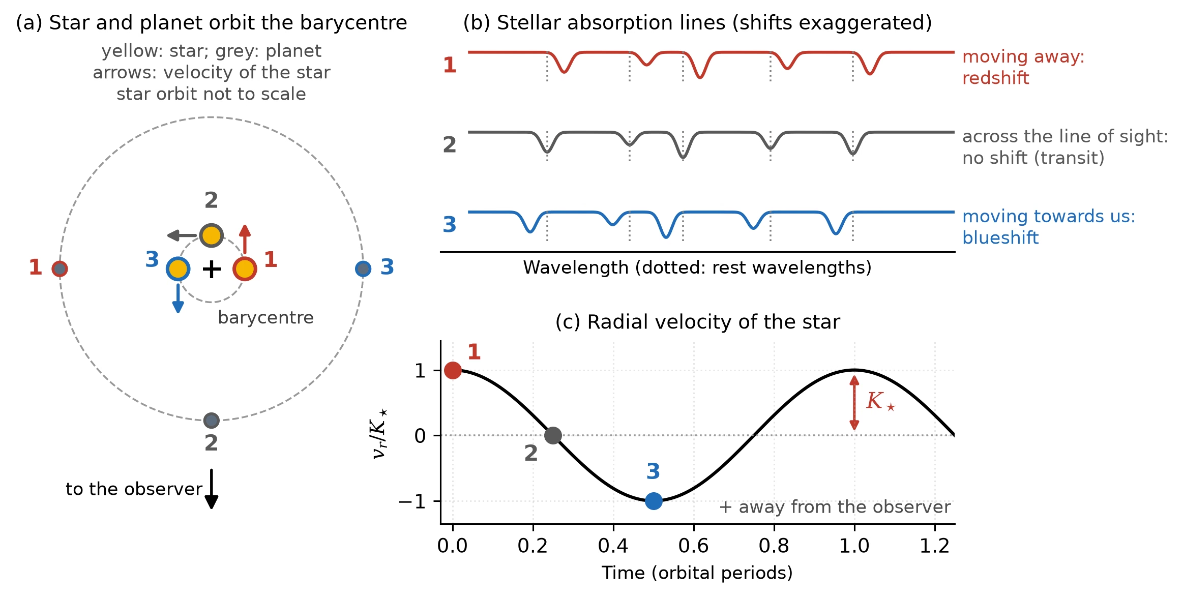
../_images/radial_velocity_geometry.avif — Fig. 13.2 Geometry of the radial velocity method. (a) Top-down view of a star and its planet on circular orbits about their common barycentre, with the observer towards the bottom; the orbit of the star is enlarged for visibility. The numbers mark three phases: (1) the star moves away from the observer, (2) the star moves across the line of sight, where the planet transits if the orbit is edge-on, and (3) the star moves towards the observer. (b) A stretch of the stellar absorption spectrum at the three phases, with the rest wavelengths dotted. The shifts are exaggerated: for $K_\star = 12.5$ m s$^{-1}$ the true shift is $\Delta\lambda/\lambda = v_r/c \approx 4 \times 10^{-8}$. (c) The radial velocity of the star over one orbit in units of $K_\star$, positive away from the observer, with the three phases marked. Course-original figure.#

Derived from Kepler’s third law and momentum conservation, the semi-amplitude for an orbit of eccentricity $e$ and inclination $i$ is

\[ K_\star = \left(\frac{2\pi G}{P}\right)^{1/3} \frac{m_p \sin i}{(M_\star + m_p)^{2/3}} \frac{1}{\sqrt{1 - e^2}}, \]

Around the Sun, a Jupiter analogue produces $K_\star \approx 12.5$ m/s, Saturn at $9.5$ AU produces $2.8$ m/s, and Earth at 1 AU produces $0.09$ m/s.

Instrumental precision has improved by two orders of magnitude over three decades, from 10 m/s with ELODIE to 1 m/s with HARPS [Mayor et al., 2003] and 10 cm/s with ESPRESSO [Pepe et al., 2021]. Precision is now limited by stellar noise, velocity jitter at the 10 cm/s to 1 m/s level from granulation, oscillations, and starspots, requiring activity diagnostics or long baselines to mitigate.

Because radial velocities constrain only $m_p \sin i$, a face-on system ($i = 0$, $\sin i = 0$) produces no Doppler signal while an edge-on system ($i = 90^\circ$, $\sin i = 1$) yields the true mass. This $m \sin i$ degeneracy prevents distinguishing a low-mass edge-on planet from a more massive inclined planet until inclination is measured independently from transits (where $\sin i \approx 1$), astrometry, or direct imaging.

Radial velocity surveys are biased toward massive planets on short orbits around bright, quiet stars, requiring at least a decade of baseline for long-period Jupiter analogues. Because optical M dwarfs have complex molecular spectra and rapidly rotating F dwarfs lack sharp lines, surveys achieve their strongest yields around quiet G and K stars in the 5 to 10 parsec neighbourhood.

Fig. 13.3 compares these semi-amplitudes with the instrument precisions.

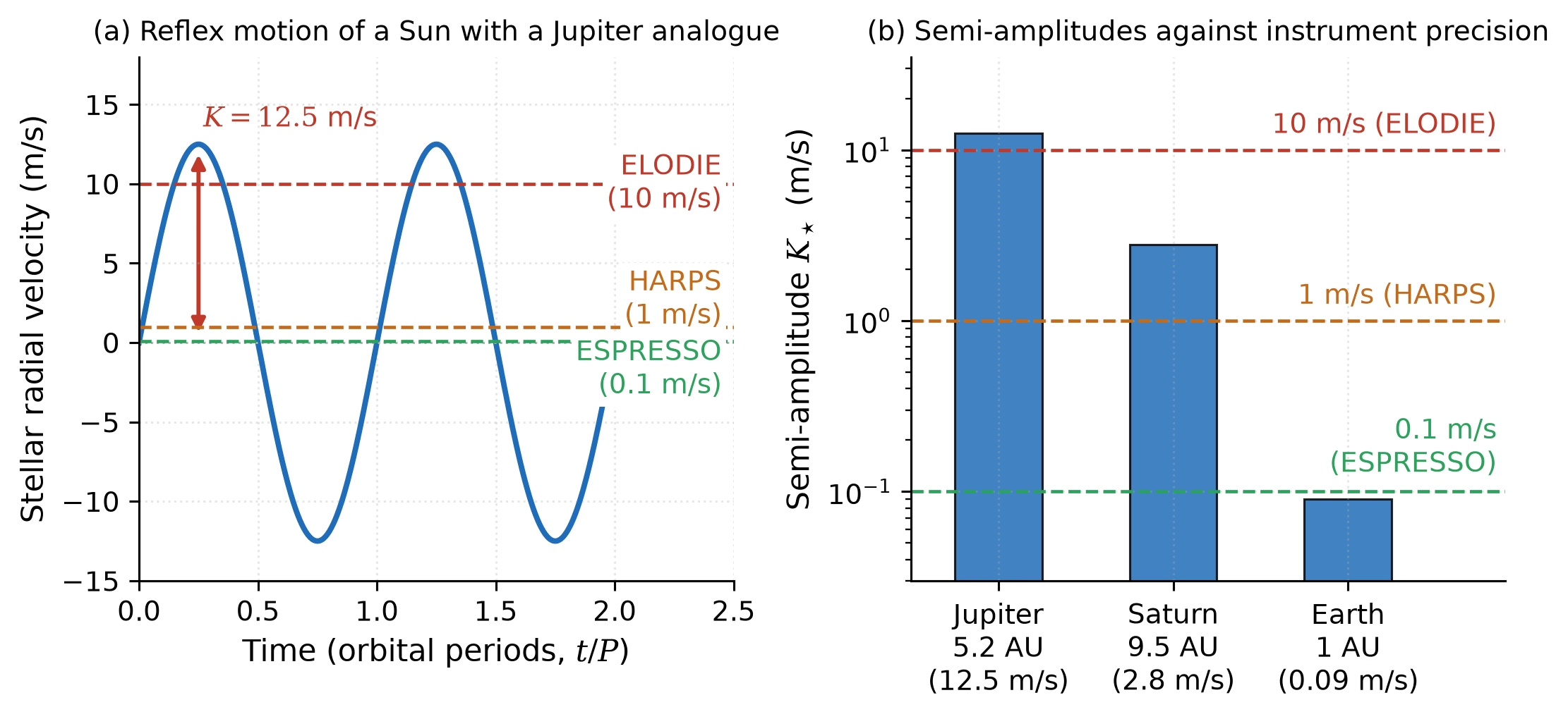
../_images/radial_velocity_signal.avif — Fig. 13.3 (a) The stellar reflex velocity of a Sun with a Jupiter analogue over two orbital periods, semi-amplitude $K_\star = 12.5$ m s$^{-1}$, against the instrument precisions of ELODIE (10 m s$^{-1}$), HARPS (1 m s$^{-1}$) and ESPRESSO (0.1 m s$^{-1}$). (b) The semi-amplitudes of a Jupiter analogue (12.5 m s$^{-1}$), Saturn at 9.5 AU (2.8 m s$^{-1}$) and Earth at 1 AU (0.09 m s$^{-1}$) against the same precisions: an Earth analogue sits below the instrumental floor and within the stellar noise. Course-original figure.#

13.1.3. Transit method#

A transit occurs when an exoplanet passes in front of its host star, blocking a fraction of stellar light (Fig. 13.4). The fractional flux drop for a planet of radius $R_p$ crossing a star of radius $R_\star$ is:

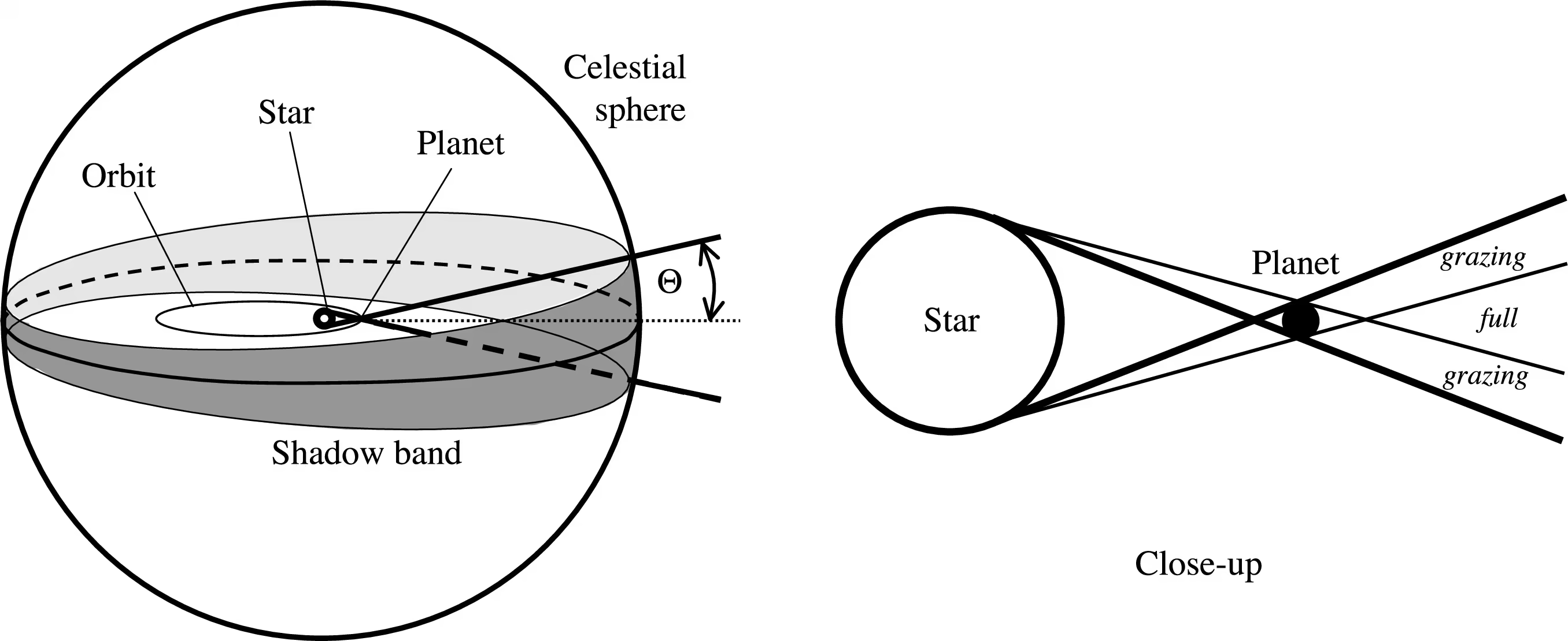
\[ \delta = \frac{\Delta F}{F} = \left(\frac{R_p}{R_\star}\right)^2. \]

../_images/transit_geometry.avif — Fig. 13.4 Geometry of a transit. **Left:** the orbit, viewed from above, defines a “shadow band” within which an observer sees transits. The half-angle of the band is $\Theta \approx (R_\star + R_p)/r$, where $r$ is the instantaneous star-planet distance. **Right:** detail of grazing and full transits relative to the stellar limb. The probability that a randomly oriented orbit produces a visible transit scales as $R_\star / a$. From the Winn (2010) review [Winn, 2010].#

For a Jupiter-radius planet around a Sun-like star, the transit depth is $\delta \approx 1\%$, measurable from the ground. For an Earth-Sun analogue, $\delta \approx 8.4 \times 10^{-5}$ (84 parts per million), achievable only from space. Around an M dwarf ($R_\star \approx 0.15\,\Rsun$), an Earth-radius planet yields $\delta \approx 4 \times 10^{-3}$ (4000 ppm), favouring M-dwarf systems for characterisation.

Four contact times ($t_\mathrm{I}$ through $t_\mathrm{IV}$) in the light curve (Fig. 13.5) constrain the orbital inclination $i$, impact parameter $b$, and planetary radius. The transit is also shaped by limb darkening, where the stellar limb appears dimmer because lines of sight probe cooler upper photospheric layers.

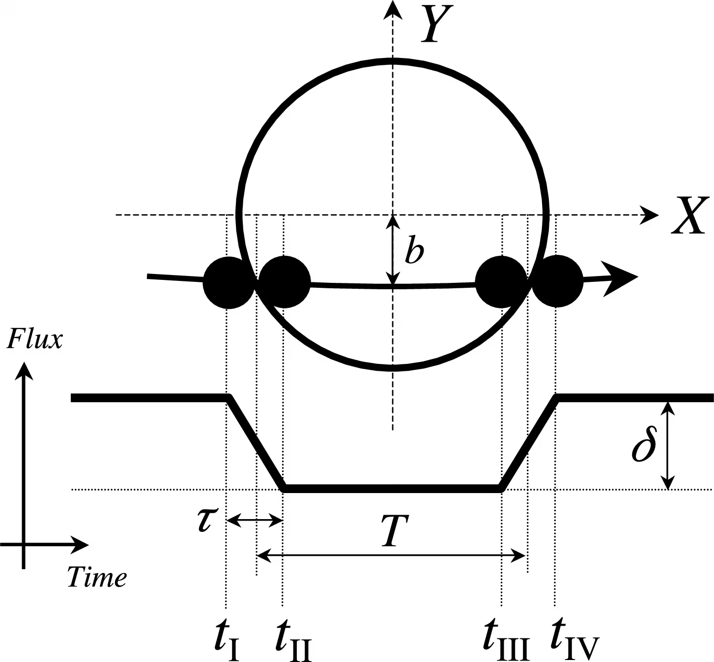
../_images/transit_lightcurve_schematic.avif — Fig. 13.5 Schematic of a transit light curve. The four contact times $t_\mathrm{I}$ through $t_\mathrm{IV}$ define the ingress, total duration, and egress. The depth $\delta = (R_p / R_\star)^2$ gives the planet’s radius if the stellar radius is known; the duration and ingress shape constrain the impact parameter $b$ and the orbital geometry. The flat bottom assumes a uniform source; in practice the curved bottom of a real transit reveals limb darkening of the host star. From Winn [2010].#

An orbit transits only if aligned within an angle $\Theta \approx R_\star / a$ of our line of sight. This probability is $\sim 0.005$ (one in 200) for an Earth-Sun analogue and $\sim 0.1$ (ten per cent) for a hot Jupiter at 0.05 AU, biasing detections toward short periods. Space photometry reaches parts-per-million precision (Fig. 13.6).

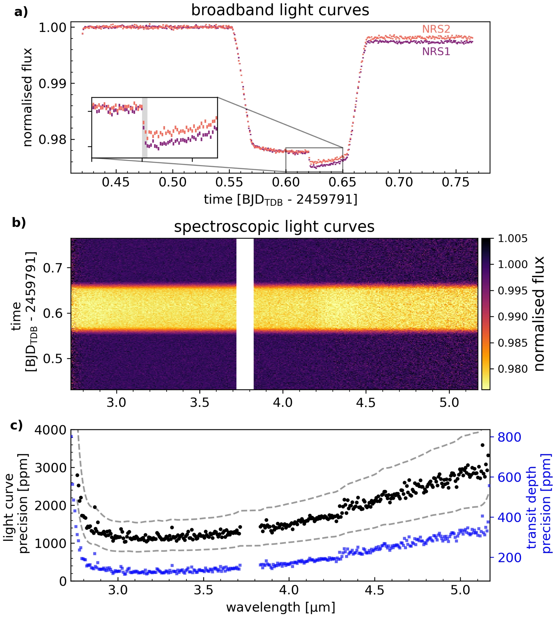
../_images/jwst_transit_lightcurve.avif — Fig. 13.6 Modern transit photometry pushed to its current limit, from Figure 1 of Alderson *et al.* [2023]. Panel a is the raw, uncorrected broadband transit light curve of the hot Saturn **WASP-39 b** ($0.28\,\Mjup$) observed with the two JWST NIRSpec G395H detectors, NRS1 (purple) and NRS2 (red); normalised flux against time in days. The inset magnifies a drop in flux (grey band) caused by a tilt of a primary-mirror segment, which leaves the two detectors offset from each other for the rest of the observation. Panel b is the same data resolved by wavelength: each column is one spectroscopic light curve, with time on the vertical axis and normalised flux as the colour. The white stripe at $3.72$–$3.82$ $\mu$m is the gap between the two detectors. Panel c is the precision reached in each spectroscopic bin: black points and the left axis are the scatter of the light curve, between about $1100$ ppm near $3.2$ $\mu$m and about $3000$ ppm near $5.1$ $\mu$m, and the two grey dashed curves are one and two times the photon noise. Blue points and the right axis are the resulting precision on the transit depth, about $200$ ppm at the blue end and about $600$ ppm at the red end. The strongest transmission feature of WASP-39 b, the $\mathrm{CO_2}$ band near $4.3$ $\mu$m, is about $1300$ ppm deep (Fig. 13.41), so a single spectroscopic bin now resolves it.#

Kepler monitored 150,000 stars to deliver the first statistical sample of small exoplanets [Borucki et al., 2010]. TESS surveys bright nearby stars for atmospheric follow-up, while CHEOPS refines planet radii. PLATO is designed to detect Earth-sized planets in the habitable zones, the orbital distances at which a rocky planet could plausibly sustain liquid surface water, of bright Sun-like stars [Rauer et al., 2014].

13.2. Blackboard derivation: Transit depth, radial velocity, and bulk density#

Blackboard derivation: Transit depth, radial velocity, and bulk density

This derivation is the central conceptual payoff of the lecture. Both the transit method and the radial velocity method have an obvious individual limitation: a transit alone gives a radius but not a mass, and a radial velocity alone gives only a minimum mass. Combining the two breaks the degeneracy, gives both quantities for the same planet, and turns an exoplanet detection into a physical object whose internal composition can be discussed. We work through this in four steps and then combine the two observables.

Fig. 13.7 shows the two observables side by side: the planet of radius $R_p$ crossing the stellar disc of radius $R_\star$, and the flux dip $\Delta F$ it produces in the light curve.

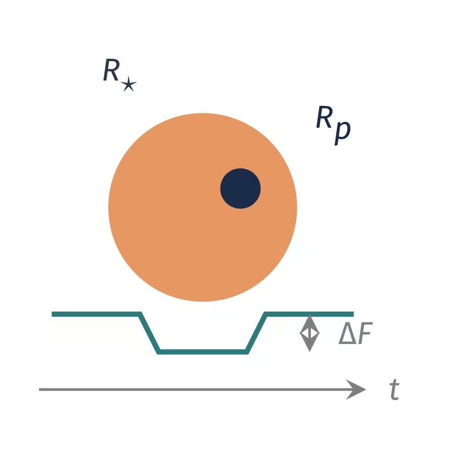
../_images/board_sketch_l13.avif — Fig. 13.7 Setup sketch of the board derivation of the planet bulk density: a planet of radius $R_p$ transits a star of radius $R_\star$, and the light curve below drops by $\Delta F$ for the duration of the transit. Course-original figure.#

Step 1: Transit depth. Treat the star as a uniformly bright disk of radius $R_\star$ and the planet as an opaque circular disk of radius $R_p$. When the planet is fully in front of the star, the area blocked is $\pi R_p^2$ and the area of the star is $\pi R_\star^2$. The fractional flux drop is therefore the ratio of areas:

\[ \frac{\Delta F}{F} = \frac{\pi R_p^2}{\pi R_\star^2} = \left(\frac{R_p}{R_\star}\right)^2. \]

The depth is the directly measured observable. If we know the stellar radius (typically from spectroscopy combined with stellar evolution models, or in the best cases from interferometric angular diameters and parallax distances), we immediately get the planet radius. Limb darkening, ingress shape, and orbital eccentricity all introduce $\sim$10% level corrections, but the leading-order picture is just the area ratio.

Step 2: The star’s orbit about the barycentre. Now we attack the dynamical side. The two bodies orbit their common centre of mass. Let $a$ denote the relative (planet-to-star) semi-major axis, and let $a_\star$ and $a_p$ denote the distances of the star and planet from the barycentre, with $a = a_\star + a_p$. Conservation of momentum at any instant requires

\[ M_\star a_\star = m_p a_p, \]

so $a_\star = (m_p/(M_\star + m_p))\,a$ and $a_p = (M_\star/(M_\star + m_p))\,a$. Both bodies move on circles (assuming a circular orbit) around the barycentre with the same orbital period $P$, and the orbital speed of the star is

\[ v_\star = \frac{2\pi a_\star}{P} = \frac{m_p}{M_\star + m_p} \cdot \frac{2\pi a}{P}. \]

We do not measure $v_\star$ directly: we measure only the line-of-sight projection $v_\star \sin i$, where $i$ is the inclination of the orbit normal to our line of sight. The maximum line-of-sight reflex velocity is therefore

\[ K_\star = v_\star \sin i = \frac{m_p \sin i}{M_\star + m_p} \cdot \frac{2\pi a}{P}. \]

Step 3: Kepler removes $a$: the semi-amplitude. To eliminate $a$ in favour of measurable quantities we use Kepler’s third law for the relative semi-major axis,

\[ a^3 = \frac{G(M_\star + m_p) P^2}{4\pi^2}, \qquad a = \left(\frac{G(M_\star + m_p) P^2}{4\pi^2}\right)^{1/3}. \]

Substituting into $K_\star$ gives

\[ K_\star = \frac{m_p \sin i}{M_\star + m_p} \cdot \frac{2\pi}{P} \cdot \left(\frac{G(M_\star + m_p) P^2}{4\pi^2}\right)^{1/3} = \left(\frac{2\pi G}{P}\right)^{1/3} \frac{m_p \sin i}{(M_\star + m_p)^{2/3}}. \]

For the case $m_p \ll M_\star$, which holds for almost all known exoplanets, we can approximate $(M_\star + m_p)^{2/3} \approx M_\star^{2/3}$. For an eccentric orbit a factor of $1/\sqrt{1 - e^2}$ multiplies the right-hand side. The full expression in the literature includes that eccentricity factor:

\[ K_\star = \left(\frac{2\pi G}{P}\right)^{1/3} \frac{m_p \sin i}{M_\star^{2/3}} \frac{1}{\sqrt{1 - e^2}}. \]

Two things should be clear from this expression. First, $K_\star \propto P^{-1/3}$, so short-period planets give a larger reflex than long-period planets at the same mass. Second, $K_\star \propto m_p \sin i$, so a radial velocity measurement alone gives only the minimum mass $m_p \sin i$, not the true mass $m_p$.

Step 4: Numbers: Jupiter around the Sun. Take $P = 11.86$ yr $= 3.743 \times 10^{8}$ s, $m_p = 1.898 \times 10^{27}$ kg, $M_\odot = 1.989 \times 10^{30}$ kg, $\sin i = 1$ and $e = 0$. In SI units, $(2\pi G/P)^{1/3} = (1.120 \times 10^{-18})^{1/3} = 1.039 \times 10^{-6}$ and $m_p/M_\odot^{2/3} = 1.898 \times 10^{27}/1.582 \times 10^{20} = 1.200 \times 10^{7}$, so $K_\star = 12.5$ m/s. The same steps give $K_\star = 0.09$ m/s for Earth, the values quoted for the radial velocity method above.

Combining the two observables. Suppose now that the same planet both transits and produces a measurable radial velocity signal. The transit immediately tells us that the orbital plane is nearly edge-on: the impact parameter is small and $\sin i \approx 1$ to better than a few per cent (a non-grazing transit requires $i$ within roughly $R_\star / a$ of $90^\circ$). This single piece of information collapses the $m_p \sin i$ degeneracy: with $\sin i \approx 1$ the inferred $m_p \sin i$ is the true mass $m_p$. We now have, for the same object:

$R_p$ from the transit depth and the stellar radius.
$m_p$ from the radial velocity semi-amplitude, the orbital period, and the stellar mass.

The bulk density follows immediately from elementary geometry:

\[ \bar{\rho}_p = \frac{m_p}{\frac{4}{3}\pi R_p^3} = \frac{3 m_p}{4\pi R_p^3}. \]

This is the central observational quantity that turns an abstract exoplanet detection into a physically meaningful object. A density of about $5.5$ g/cm$^3$ matches an Earth-like silicate-iron rocky composition. A density of about $1.3$ g/cm$^3$ matches Jupiter and is consistent with a hydrogen-helium envelope around a small dense core. A density of $0.5$ g/cm$^3$, lower than water, indicates an inflated or low-mass H/He envelope. A density of $1$–$3$ g/cm$^3$ for a planet of $2$ to $4\,\Rearth$ is typical of “sub-Neptunes” and indicates a substantial water-ice or H/He volatile component on top of a rocky core. Without the joint transit-plus-RV measurement, we cannot tell any of these apart (Fig. 13.8 collects the empirical mass-radius relation across the four major compositional regimes).

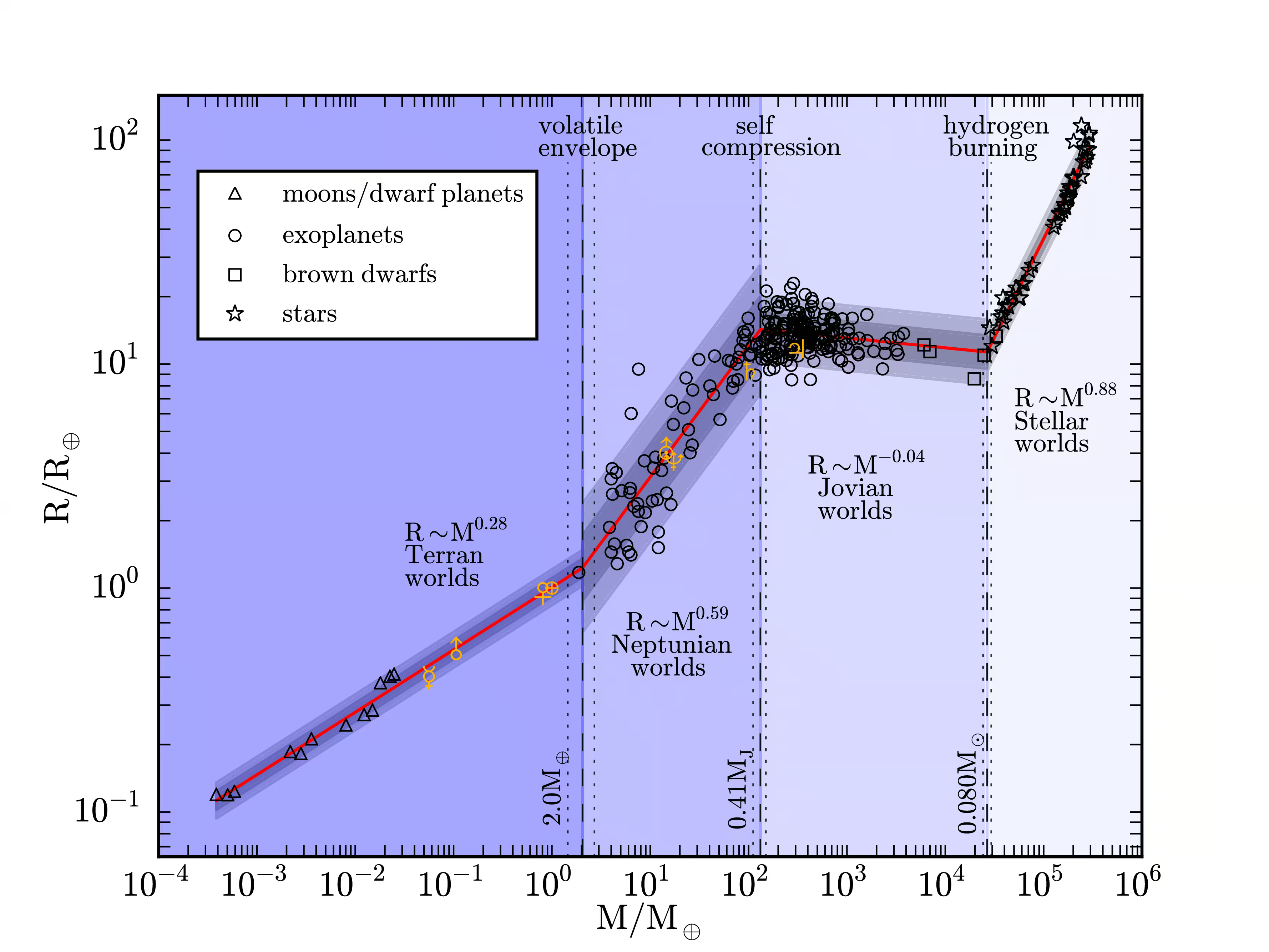
../_images/chenkipping_mass_radius.avif — Fig. 13.8 Empirical mass-radius relation across the full range of solar-system bodies, exoplanets, brown dwarfs, and stars, from Chen and Kipping [2017]. The shaded regions mark four distinct compositional regimes: terran ($M \lesssim 2\,\Mearth$, scaling roughly as $R \propto M^{0.28}$), Neptunian ($2\,\Mearth \lesssim M \lesssim 0.4\,\Mjup$, $R \propto M^{0.59}$), Jovian ($0.4\,\Mjup \lesssim M \lesssim 80\,\Mjup$, $R \propto M^{-0.04}$, where electron degeneracy and self-compression flatten the relation), and stellar ($M > 80\,\Mjup$, hydrogen burning sets in). Each break corresponds to a different dominant pressure source. The “Neptunian” segment is the modern compositional location of the sub-Neptune family, the population that has no analogue in the solar system.#

The pedagogical message is this. The transit-plus-RV combination is the single piece of observational machinery that took exoplanet science from an exotic claim about a few hot Jupiters in 1995 to a quantitative compositional census of thousands of planets by 2020. Every demographic structure we will discuss in Part 2, including the radius valley and the sub-Neptune family, exists as a discovery only because we can measure both $R_p$ and $m_p$ for the same object.

13.3. Part 1, continued: imaging, astrometry and timing#

13.3.1. Direct imaging#

Direct imaging spatially separates planetary photons from stellar light on a detector. Contrast reaches $10^{-9}$ for a Jupiter at 5 AU and $10^{-10}$ for an Earth analogue at 10 pc, at angular separations of $0.1$ arcsecond.

Adaptive optics correct atmospheric turbulence with deformable mirrors to achieve diffraction-limited resolution. Coronagraphs suppress central starlight, while angular differential imaging (ADI) and spectral differential imaging (SDI) subtract residual stellar speckles.

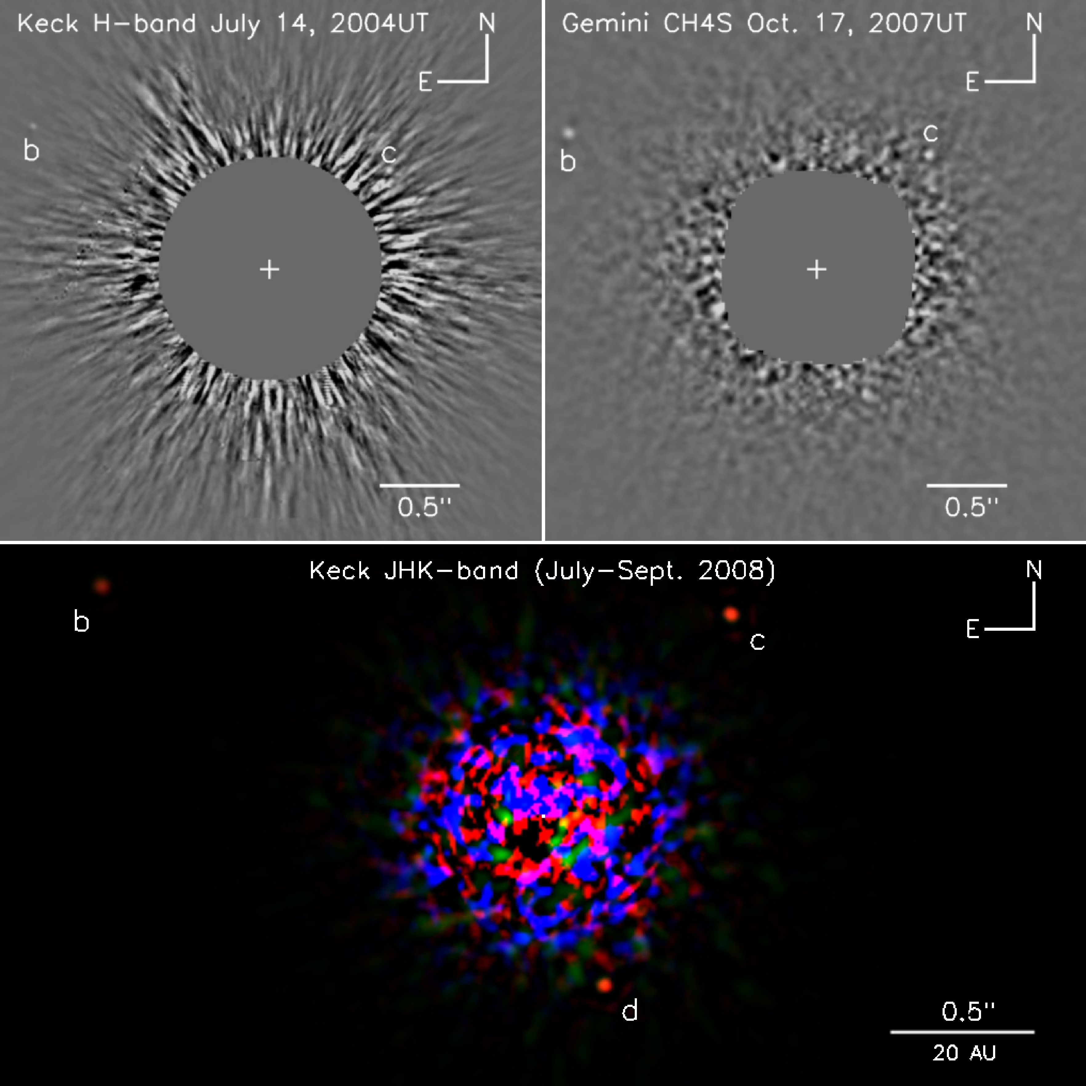
../_images/hr8799_discovery.avif — Fig. 13.9 Discovery image of the **HR 8799** planetary system from Marois *et al.* [2008], showing planets d, c, and b at projected separations of $24$, $38$, and $68$ AU after angular differential imaging PSF subtraction. The three were found in 2004 to 2008 Keck and Gemini observations; planet e, at $\sim 14$ AU, was added in 2010, and the four young giants have masses of roughly $5$–$10\,\Mjup$ and span orbital separations of $14$–$68$ AU.#

Because young giant planets ($\lesssim 100$ Myr old) still radiate formation heat, direct imaging favours massive ($> 1\,\Mjup$), wide-orbit ($> 10$ AU) giants such as HR 8799 [Marois et al., 2008] (Fig. 13.9) and $\beta$ Pictoris b [Lagrange et al., 2010] (Fig. 13.10).

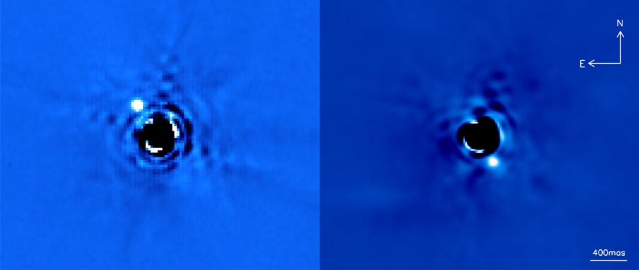
../_images/betapic_imaging.avif — Fig. 13.10 Direct image of $\beta$ Pictoris b from Lagrange *et al.* [2010], showing clear orbital motion between 2003 (left) and 2009 (right) that confirms a bound $\sim 9\pm 3\,\Mjup$ companion at $\sim 9$ AU. The host star also harbours an extensively imaged debris disk and an interior second giant planet (c) at $\sim 2.7$ AU.#

PDS 70 contains the first planets detected directly inside a cleared protoplanetary disk gap [Haffert et al., 2019, Keppler et al., 2018]. Accretion onto b and c produces shock H$\alpha$ emission confirming planet-disk interaction models [Haffert et al., 2019] (Lecture 2; Fig. 13.11 and Fig. 13.12).

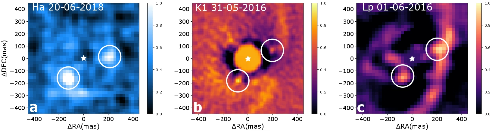
../_images/pds70bc_haffert.avif — Fig. 13.11 Detection of PDS 70 b and c in three epochs and three wavelength bands, from Figure 2 of Haffert *et al.* [2019]. All three panels show the same field: offset in right ascension against offset in declination, both in milliarcseconds, with the star at the origin (white star symbol) and the two planets marked by white circles. Each panel has its own colour bar, normalised from 0 to 1. Panel a is the MUSE H$\alpha$ detection map of 20 June 2018, after removal of the direct and scattered starlight; the band just south of PDS 70 b is most likely an artefact of the MUSE image slicer. Panel b is the SPHERE/IRDIS K1-band image of 31 May 2016 after angular differential imaging. Panel c is the NACO L$'$-band image of 1 June 2016, in which PDS 70 c is blended with the disk because the point spread function is broad at that wavelength. The H$\alpha$ emission of PDS 70 b and of the newly discovered PDS 70 c is interpreted as accretion shock luminosity from gas that falls onto the planets, which is evidence that two protoplanets accrete at the same time in the disk gap.#

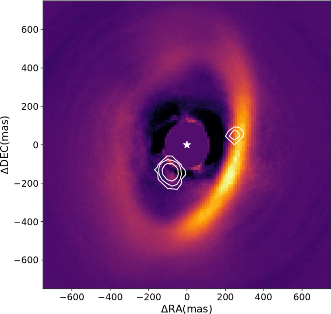
../_images/pds70_disk.avif — Fig. 13.12 Composite scattered-light image of the PDS 70 protoplanetary disk from Haffert *et al.* [2019], showing the parent disk and two embedded protoplanets (b and c) inside the cleared gap. The cleared central cavity and accreting protoplanets provide direct confirmation of planet-disk interaction models in transition disks.#

13.3.2. Astrometry#

Astrometry measures the angular reflex motion of the host star against background reference stars. The expected angular amplitude is

\[ \alpha = \frac{m_p}{M_\star} \cdot \frac{a_p}{d}, \]

where $d$ is the distance to the system. For a Jupiter analogue around the Sun at 10 pc, this is about half a milli-arcsecond, whereas for an Earth analogue it is $0.3$ micro-arcseconds. Astrometric exoplanet detection therefore demands microarcsecond precision over years to decades.

Gaia, launched in 2013, performs an all-sky astrometric survey of more than a billion stars with a final precision of $\sim 10$ microarcseconds for bright stars. This is the precision regime in which Jupiter analogues become accessible.

Early Gaia data releases provided five-parameter astrometry and orbital fits for substellar companions [Gaia Collaboration et al., 2023]. Future Gaia data releases (DR4 and DR5) will deliver astrometric time series to provide a census of long-period gas giants [Perryman et al., 2014].

Astrometry is complementary to radial velocity because it directly measures the inclination of the orbit, breaking the $m \sin i$ degeneracy without requiring a transit. A planet that produces both a Gaia astrometric signal and a radial velocity signal yields a true mass, an orbit inclination, and a complete three-dimensional orbital solution. The combination is particularly powerful for wide-orbit Jupiter analogues that fall in the blind spot of transit surveys.

Fig. 13.13 shows the amplitude against distance for the two analogues.

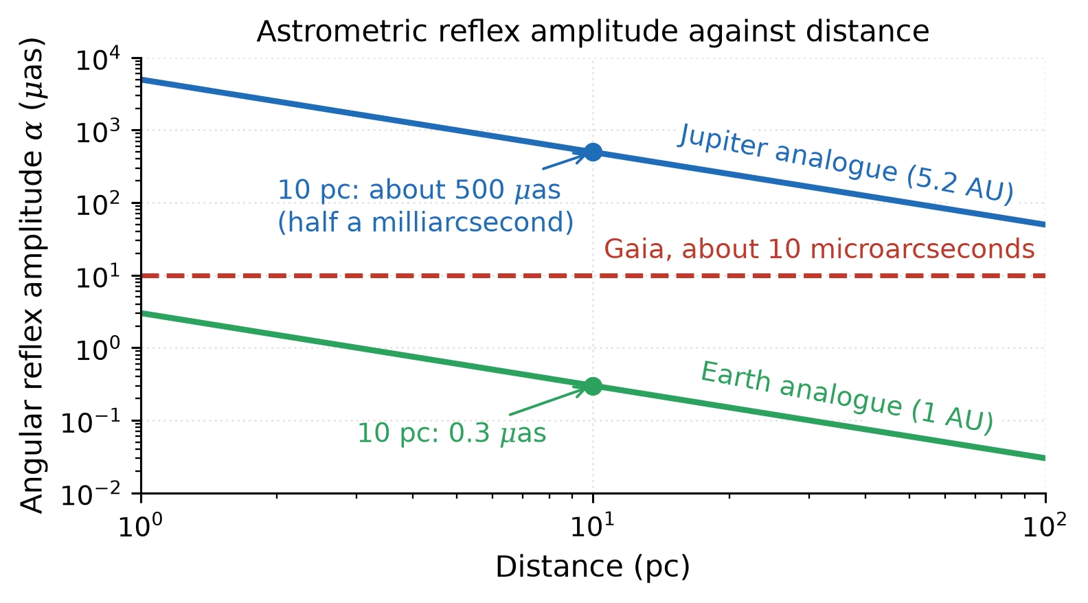
../_images/astrometric_signal.avif — Fig. 13.13 Astrometric reflex amplitude $\alpha = (m_p/M_\star)(a_p/d)$ against distance for a Jupiter analogue at 5.2 AU and an Earth analogue at 1 AU around a Sun-like star ($\alpha$ in arcseconds for $a_p$ in AU and $d$ in pc). At 10 pc the Jupiter analogue gives about 500 microarcseconds, half a milliarcsecond, and the Earth analogue 0.3 microarcseconds; the dashed line is Gaia’s final precision of about 10 microarcseconds for bright stars, the regime in which Jupiter analogues become accessible. Course-original figure.#

13.3.3. Microlensing#

In gravitational microlensing, the gravitational field of a foreground star (the lens) bends light from a distant background star, briefly magnifying its brightness. If the lens star hosts a planet, planetary gravity introduces an additional short-duration spike lasting hours to days. The amplitude and timing of this spike determine the planet’s mass and projected separation in units of the Einstein ring radius, set by the lens mass and distance.

Microlensing detects planets at distances of kiloparsecs and projected separations of $0.5$ to $10$ AU, mapping onto the snow-line region where giant planets form. The Nancy Grace Roman Space Telescope, launched in August 2026, will conduct a dedicated survey of the Galactic bulge expected to discover $\sim 1400$ bound exoplanets down to lunar-mass bodies [Penny et al., 2019].

Fig. 13.14 shows the light curve of such an event.

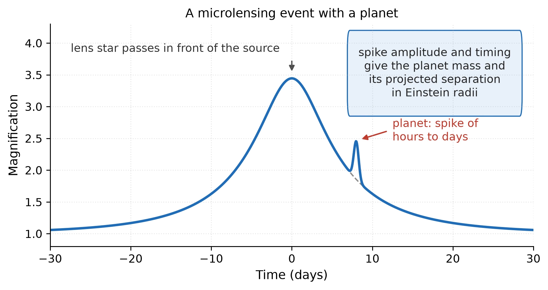
../_images/microlensing_lightcurve.avif — Fig. 13.14 A microlensing event with a planet: the magnification of a background source as the lens star passes in front of it (point-lens curve with an impact parameter of 0.3 Einstein radii and an Einstein crossing time of 15 days), with the short spike that a planet around the lens adds. The spike lasts hours to days, and its amplitude and timing give the planet’s mass and projected separation in units of the Einstein ring radius. Course-original figure.#

13.3.4. Timing methods#

When a planet has a companion in the same system, gravitational interactions periodically perturb its transit times, producing transit timing variations (TTVs) [Holman and Murray, 2005]. Because TTVs encode the masses of interacting planets, they yield a dynamical mass measurement without requiring radial velocity follow-up. This is essential for small planets around faint stars where radial velocity observations are infeasible, such as the seven planets of the TRAPPIST-1 system.

A second timing approach is pulsar timing, the technique that detected the first exoplanets [Wolszczan and Frail, 1992].

In eclipsing binaries, circumbinary planets perturb eclipse timing and can transit both stars; Kepler-16 b, found in 2011 through its transits, was the first such planet [Doyle et al., 2011].

Fig. 13.15 shows the timing signal and the three methods.

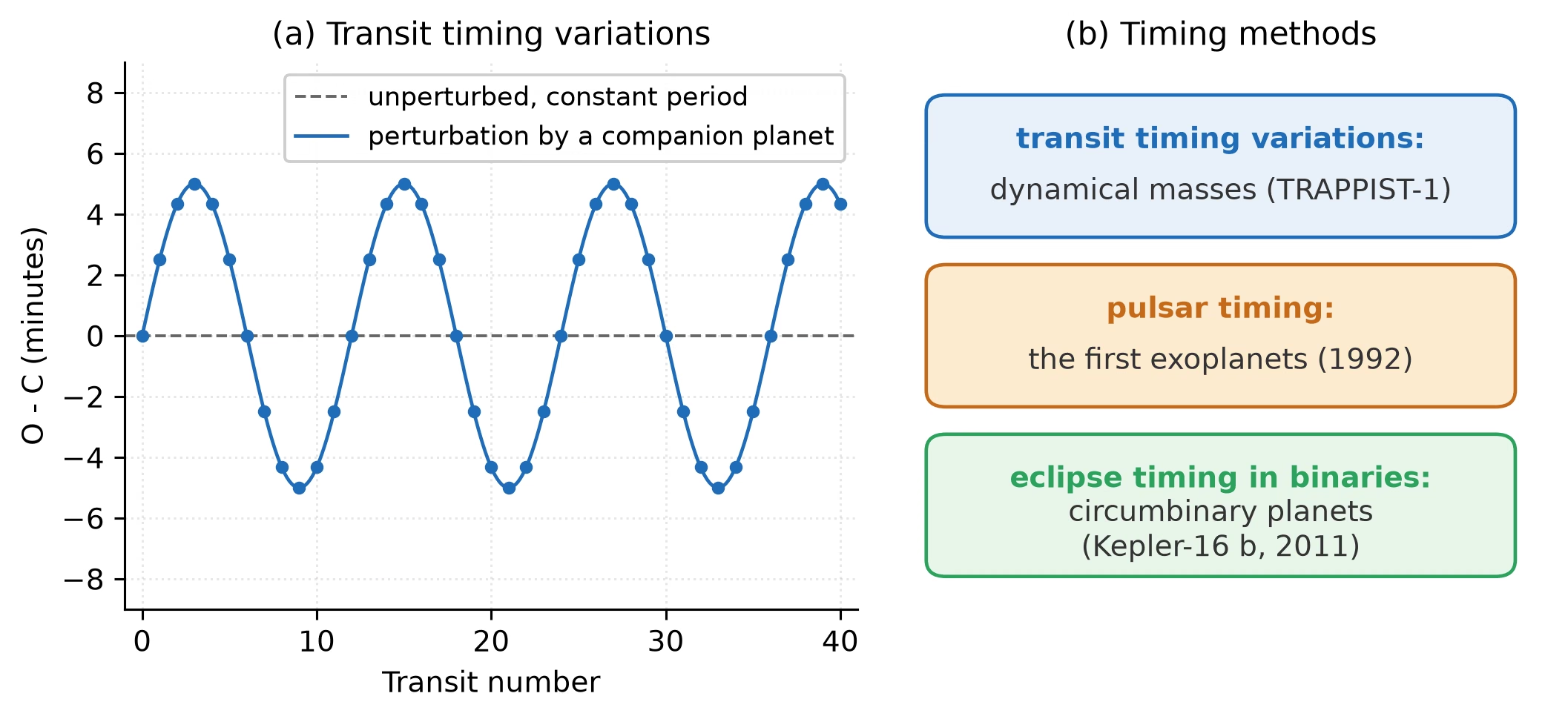
../_images/transit_timing_variations.avif — Fig. 13.15 (a) Transit timing variations: the observed minus calculated transit times of a planet perturbed by a companion oscillate about the constant-period prediction (a 5 minute amplitude over 12 transits, schematic); the amplitude and period of the variation encode the companion’s mass. (b) The three timing methods: transit timing variations give dynamical masses (TRAPPIST-1), pulsar timing found the first exoplanets (1992), and eclipse timing in binaries reveals circumbinary planets (Kepler-16 b, 2011). Course-original figure.#

13.3.5. Detection biases summary#

Each detection method introduces a detection bias, selecting planets in different regions of parameter space. Radial velocity is most sensitive to massive planets on short-period orbits (since $K \propto P^{-1/3}$) around bright Sun-like stars. Transit photometry is most sensitive to short periods (less than $\sim 100$ days) and large $R_p / R_\star$ ratios. Direct imaging detects young, self-luminous giants on wide orbits ($> 10$ AU). Astrometry is most sensitive to wide orbits matching the mission baseline. Microlensing detects planets at 1 to 10 AU at any host distance, but is unrepeatable. Timing is sensitive to compact multi-planet systems or circumbinary configurations. The distribution of confirmed exoplanets across mass and orbital period illustrates how these observational biases shape the detected population (Fig. 13.16).

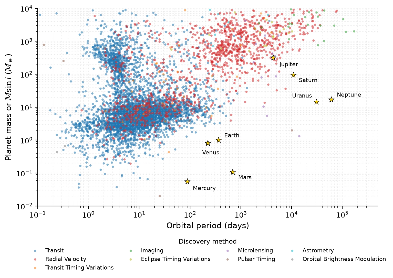
../_images/exoplanet_mass_period1.avif — Fig. 13.16 Confirmed exoplanet masses (or minimum masses $m_p \sin i$) plotted against orbital period, colour-coded by detection technique, with the solar-system planets shown for comparison. Detection biases concentrate discoveries in the high-mass and short-period regimes, leaving Earth analogues in a sparsely sampled region. Credit: NASA Exoplanet Archive [NASA Exoplanet Archive, 2026]. Course-original figure.#

The observed exoplanet archive reflects these combined biases rather than the true physical distribution. Demographic claims in Part 2 therefore require bias correction, reporting underlying occurrence rather than raw catalogue counts. This correction is reliable for Kepler, but much less certain for other surveys.

13.4. Part 2: Demographics and architectures#

13.4.1. The Kepler revolution and the TRAPPIST-1 laboratory#

On average, at least one planet exists per main-sequence star, with small planets below 4 Earth radii being the most common [Petigura et al., 2018]. Hot Jupiters occur around only 0.5% to 1% of Sun-like stars [Fressin et al., 2013]. The habitable-zone Earth-size planet occurrence rate is estimated at $\eta_\oplus \sim 0.4$ (Fig. 13.17 and Fig. 13.18) [Bryson et al., 2021].

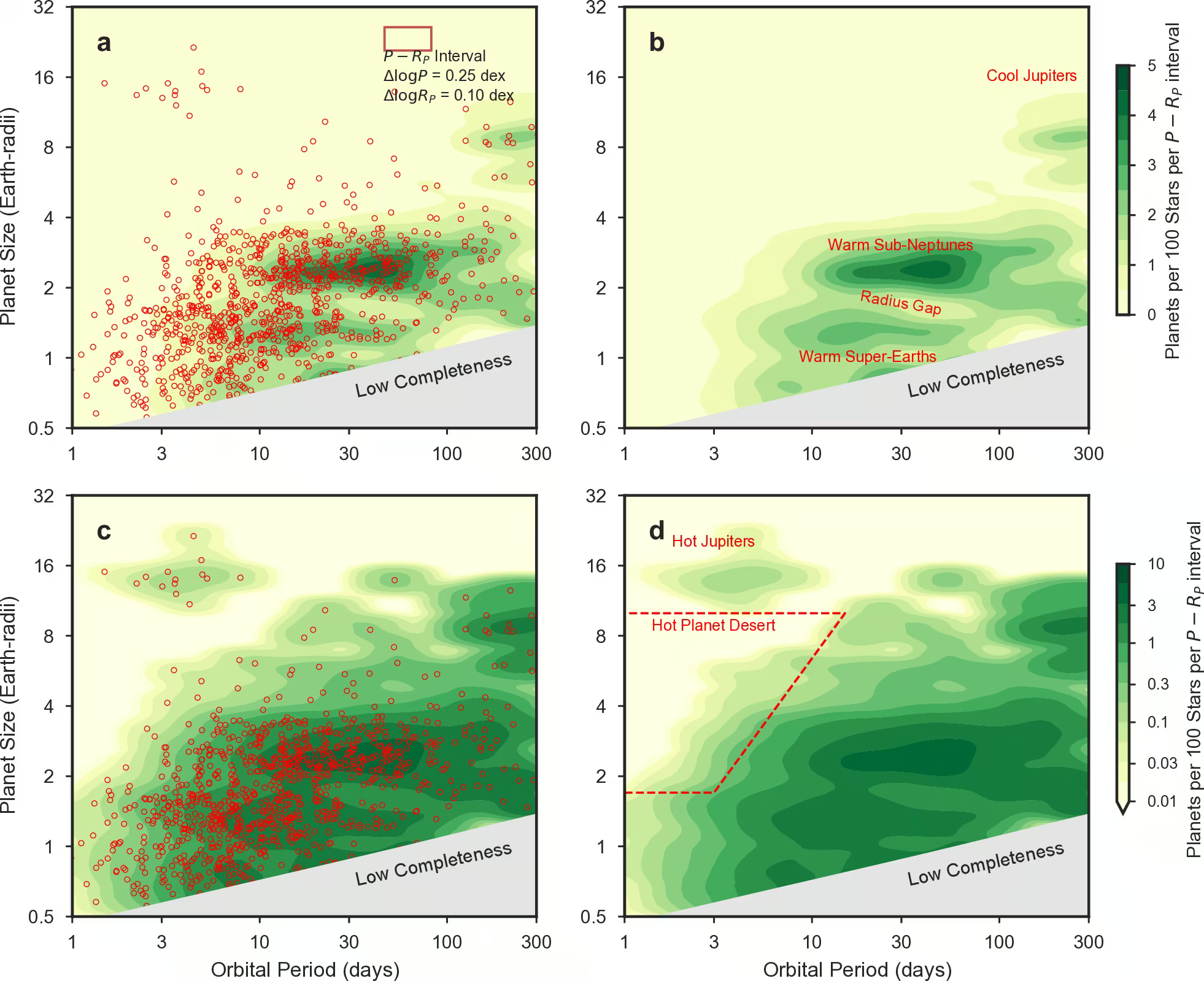
../_images/petigura_occurrence.avif — Fig. 13.17 Kepler-derived planet occurrence rates as a function of orbital period and planet size, from the California-Kepler Survey [Petigura *et al.*, 2018]. Small planets are far more common than giants at every period, and the typical Sun-like star hosts at least one small planet inside 1 AU despite Kepler’s $\sim 4$ years of baseline.#

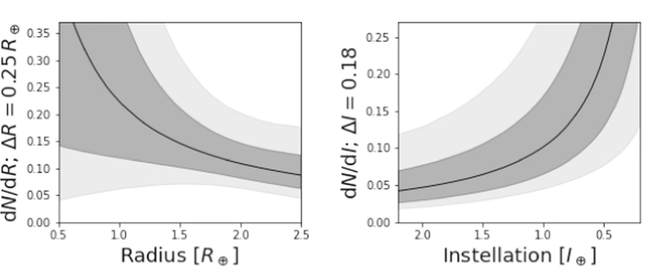
../_images/bryson_etaearth.avif — Fig. 13.18 Marginalised differential occurrence rate of small planets from Bryson *et al.* [2021], showing occurrence per unit radius $\dd N / \dd R$ ($\Delta R = 0.25\,\Rearth$, left) and per unit instellation flux $\dd N / \dd I$ ($\Delta I = 0.18$, right). Shaded bands mark 68% and 95% credible intervals, yielding central values of $\eta_\oplus \sim 0.4$ with 68% intervals of $0.2$–$0.9$ for conservative habitable-zone Earth analogues.#

The TRAPPIST-1 system hosts seven transiting Earth-sized planets within about 0.06 AU of an M8 ultra-cool dwarf at about 12 pc, three of which (e, f, g) orbit in the temperate habitable zone [Gillon et al., 2017]. The planets form a chain of mean-motion resonances, orbital periods locked near ratios of small integers, consistent with capture during an early disk-migration phase [Luger et al., 2017]. All seven planets transit (Fig. 13.19), a configuration with probability below $10^{-3}$ for random orientations, which indicates that compact M-dwarf systems are intrinsically flat, while transit timing variations yield dynamical masses (Fig. 13.20).

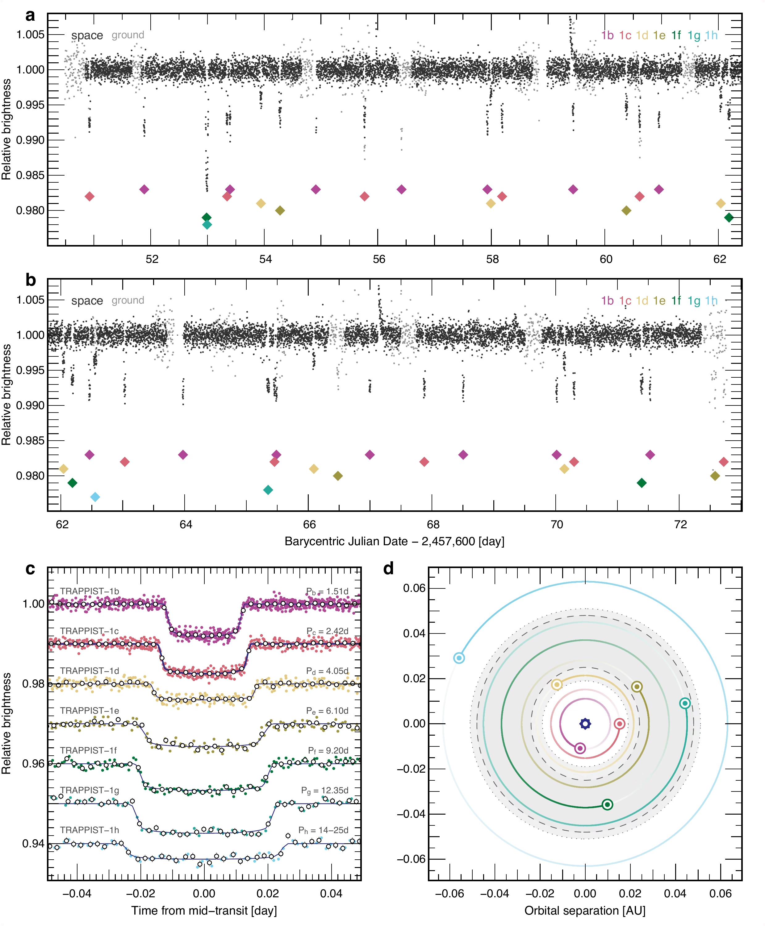
../_images/trappist1_transits.avif — Fig. 13.19 Transit light curves of the seven **TRAPPIST-1** planets (b through h) from Gillon *et al.* [2017], observed with Spitzer at $4.5\,\mu$m and ground-based facilities. Successive transit depths trace planetary sizes, showing that all seven are Earth-sized to within a factor of $\sim 1.5$.#

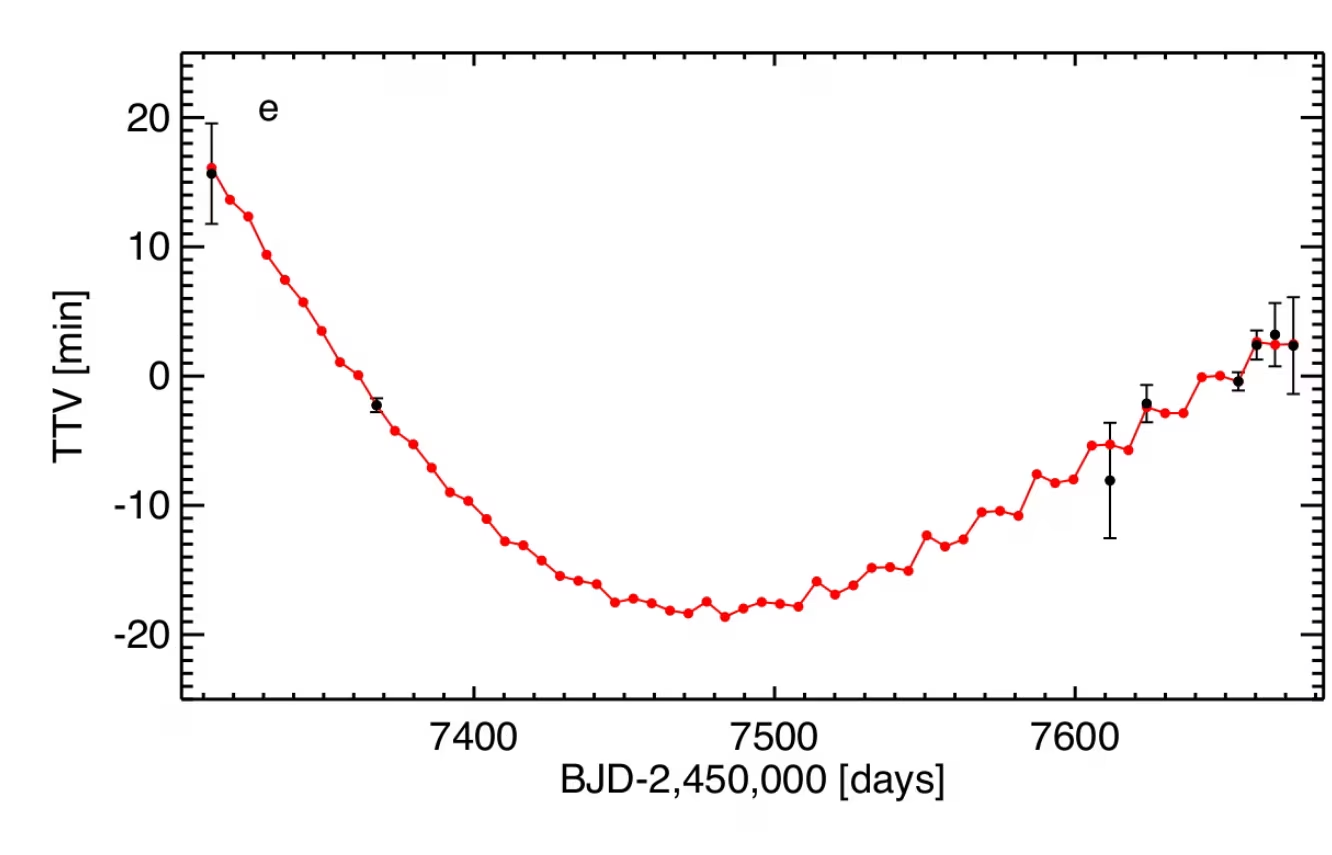
../_images/trappist1_ttvs.avif — Fig. 13.20 Transit timing variations (TTVs) of **TRAPPIST-1 e** from Gillon *et al.* [2017], with observed deviations (black points) and a dynamical model coupled to the other six planets (red curve). TTV amplitudes reaching tens of minutes over hundreds of days invert to yield **dynamical masses** for all seven planets without radial velocity measurements.#

13.4.2. The period-radius diagram#

The period-radius diagram plots orbital period against planetary radius for confirmed transiting planets (Fig. 13.21). Gas giants ($R_p > 10\,\Rearth$) include short-period hot Jupiters ($P < 10$ days). Small planets split into sub-Neptunes ($R_p \approx 2$ to $4\,\Rearth$), which have no solar system analogue, and rocky super-Earths ($R_p \approx 1$ to $1.8\,\Rearth$). The terrestrial analogue regime ($R_p \lesssim 1.5\,\Rearth$ at periods longer than $\sim 100$ days) remains largely unexplored.

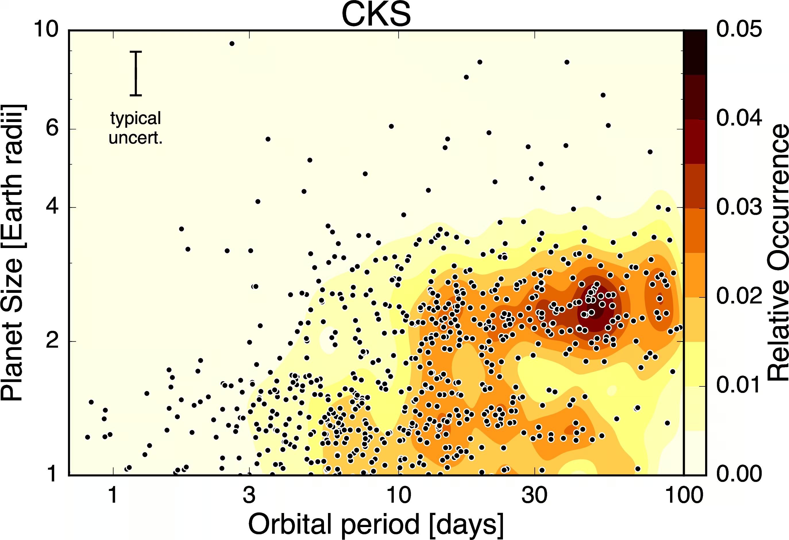
../_images/fulton_period_radius.avif — Fig. 13.21 Period-radius distribution of small Kepler planets after stellar parameter refinement and bias correction, from Fulton *et al.* [2017]. The colour scale indicates detection completeness. The clear deficit of planets at $R_p \approx 1.8\,\Rearth$ across all orbital periods is the **radius valley** or **Fulton gap**, the central empirical structure that splits the small-planet population into super-Earths and sub-Neptunes.#

13.4.3. The radius valley (Fulton gap)#

The radius valley (or Fulton gap) is a deficit of small exoplanets at $R_p \approx 1.5$ to $2\,\Rearth$ separating rocky super-Earths (peaking near $1.3\,\Rearth$) from volatile-rich sub-Neptunes (peaking near $2.4\,\Rearth$) (Fig. 13.22) [Fulton et al., 2017].

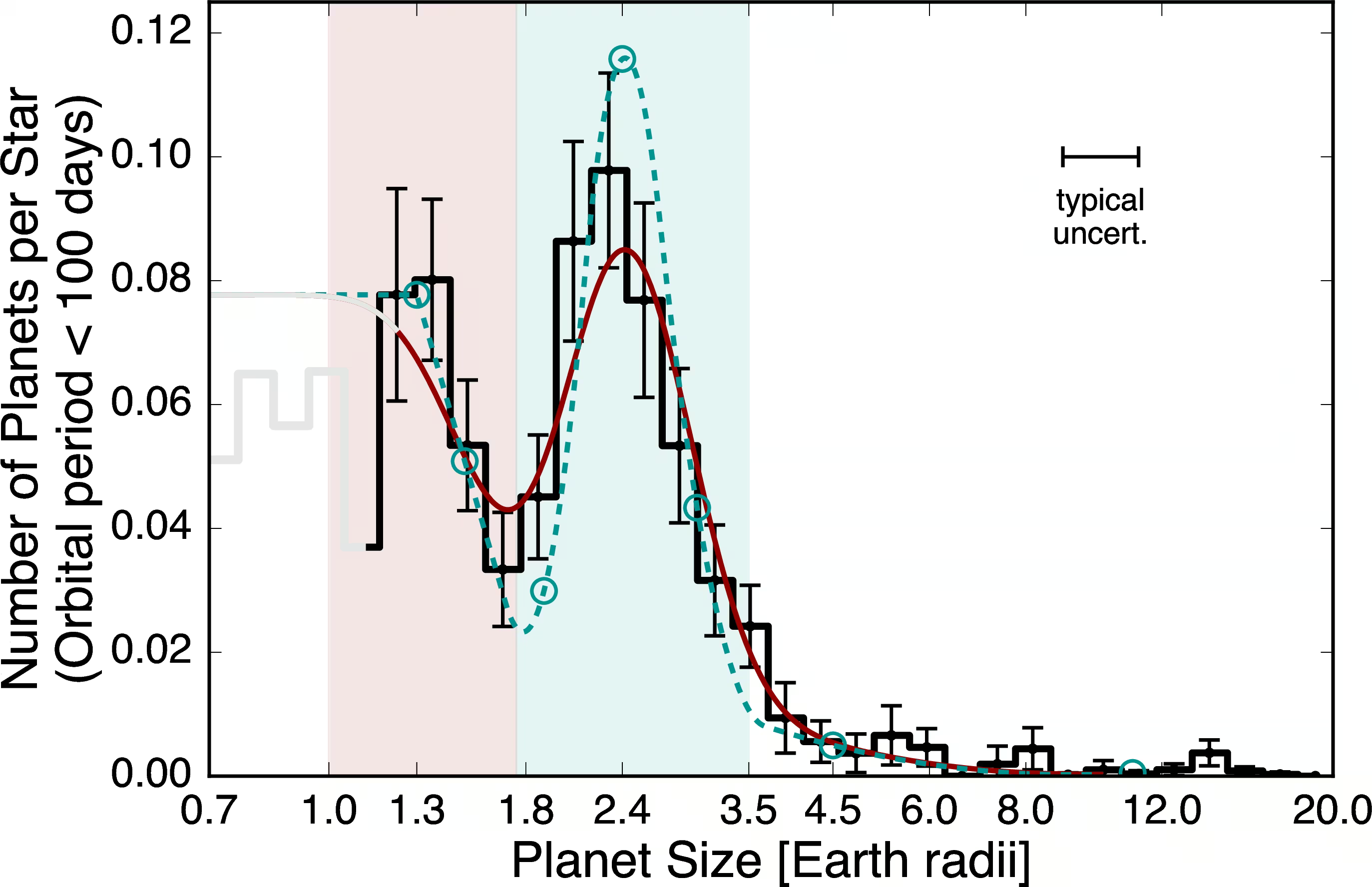
../_images/fulton_gap.avif — Fig. 13.22 The **radius valley**: histogram of planet radii in the Kepler sample after stellar parameter refinement, from Fulton *et al.* [2017]. The deficit at $R_p \approx 1.8\,\Rearth$ splits small planets into a rocky **super-Earth** group at $\sim 1.3\,\Rearth$ and a volatile-rich **sub-Neptune** group at $\sim 2.4\,\Rearth$.#

The valley is produced by atmospheric escape via two mechanisms: first, photoevaporation, where stellar XUV (ultraviolet and X-ray) radiation heats the upper envelope to drive hydrodynamic escape [Owen and Wu, 2013]. In energy-limited escape, a fraction $\epsilon \sim 0.1$ of the absorbed XUV flux converts into the gravitational work needed to lift gas out of the potential well:

\[ \dot{M} \approx \frac{\epsilon \, \pi F_\mathrm{XUV} R_p^3}{G M_p}. \]

The $R_p^3$ scaling indicates that low-density, low-mass planets are stripped most easily. For a $10\,\Mearth$ sub-Neptune with $R_p \approx 2.5\,\Rearth$ at $0.1$ AU, an initial saturated flux of $F_\mathrm{XUV} \sim 300$ W m$^{-2}$ yields $\dot{M} \sim 10^{8}$ kg s$^{-1}$, removing $\sim 3 \times 10^{23}$ kg over the $\sim 100$ Myr saturated phase to strip the envelope (Fig. 13.23).

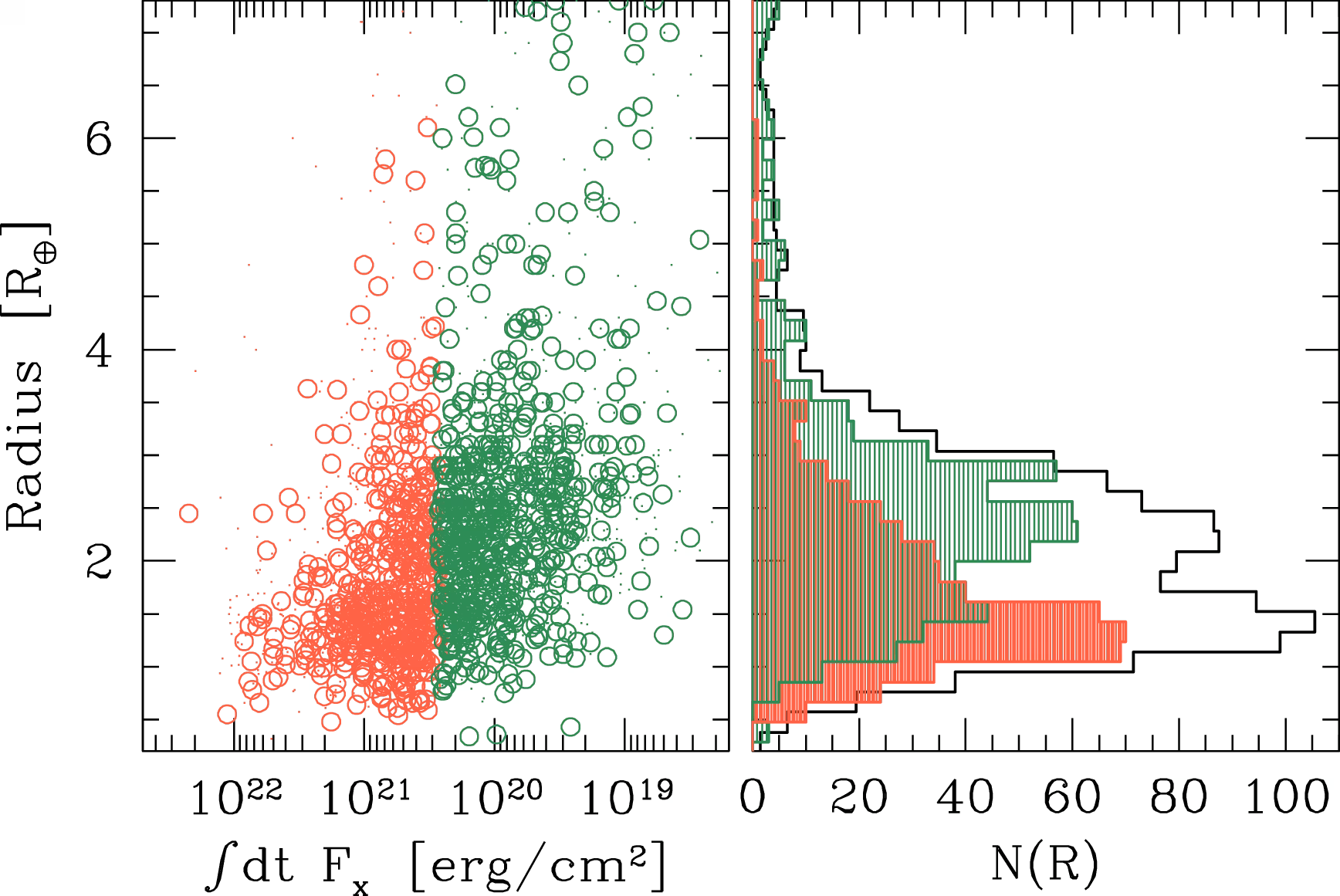
../_images/owen_evaporation_valley.avif — Fig. 13.23 Photoevaporation theory prediction of the radius valley from Owen and Wu [2013]. Planets with envelopes survive above $\sim 2\,\Rearth$, while stripped bare rocky cores settle below $\sim 1.8\,\Rearth$ to produce the observed valley.#

Fig. 13.24 shows how a young sub-Neptune loses its envelope in the photoevaporation model.

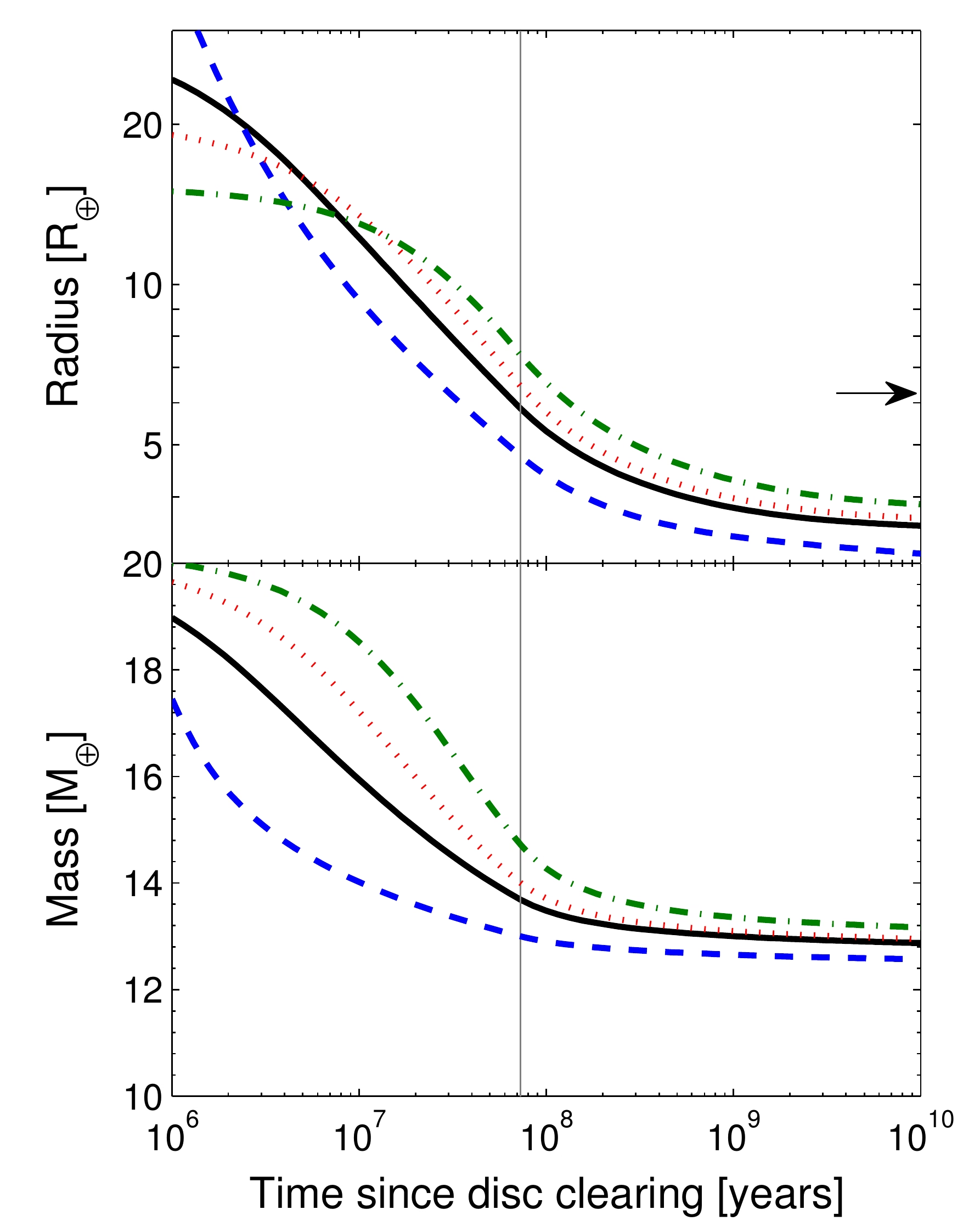
../_images/owen_xuv_massloss.avif — Fig. 13.24 Photoevaporation-driven evolution of a young sub-Neptune in the Owen and Wu [2013] model. **Top**: planetary radius as a function of time since disc clearing, for two host XUV histories (line styles) and two starting orbital separations. **Bottom**: planet mass over the same evolution. The thin vertical line marks the end of the saturated XUV phase at $\sim 100$ Myr. After this time the radius and mass plateau; planets that have lost their envelopes by then settle as bare rocky cores below the radius valley.#

The second mechanism is core-powered mass loss, where heat released from the cooling interior over hundreds of Myr powers hydrodynamic escape without external XUV flux, reproducing the gap at $\sim 1.8\,\Rearth$ (Fig. 13.25) [Ginzburg et al., 2018].

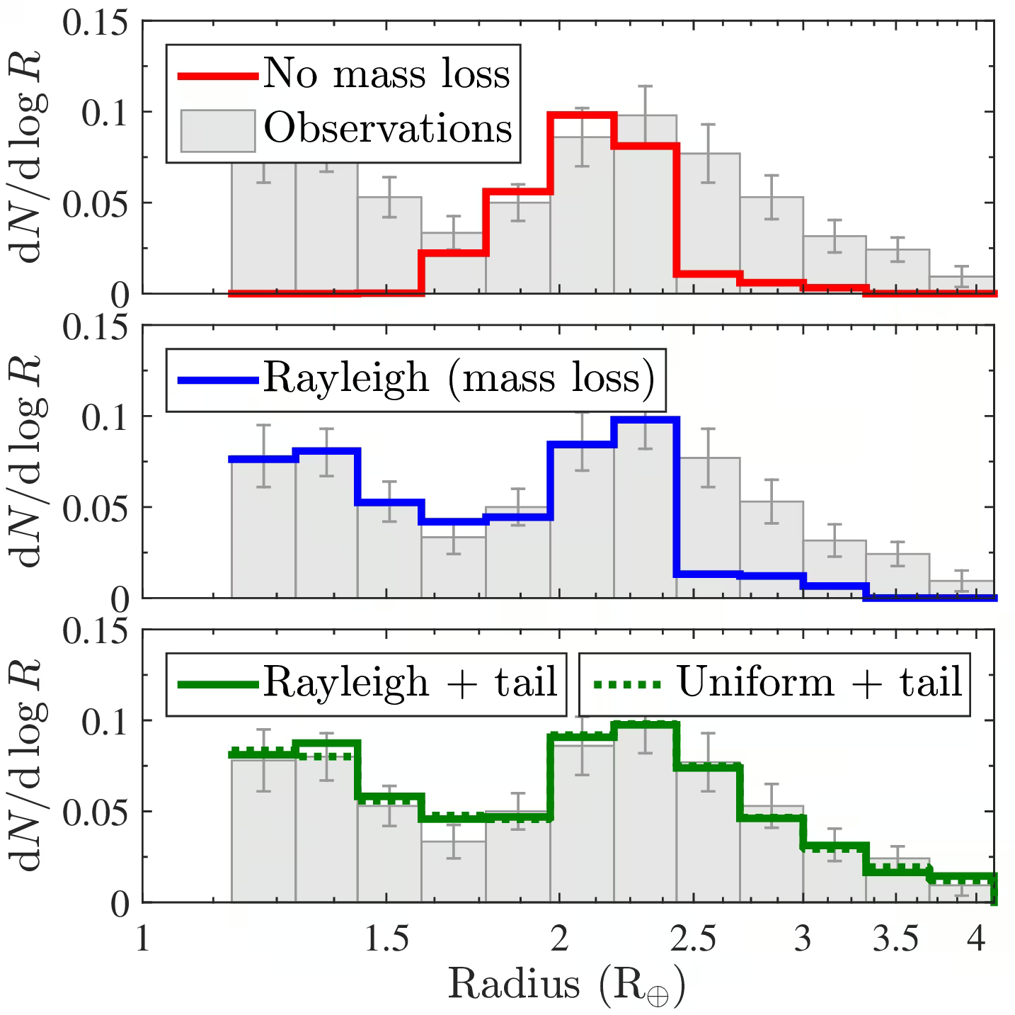
../_images/ginzburg_corepowered.avif — Fig. 13.25 Core-powered mass loss model from Ginzburg *et al.* [2018]. Envelope mass loss driven by the cooling rocky interior produces a bimodal distribution with a gap at $\sim 1.8\,\Rearth$ separating bare rocky cores from sub-Neptunes.#

Precise asteroseismic stellar radii show that the radius valley shifts to smaller radii at longer orbital periods, a negative slope consistent with both photoevaporation and core-powered mass loss (Fig. 13.26) [Van Eylen et al., 2018].

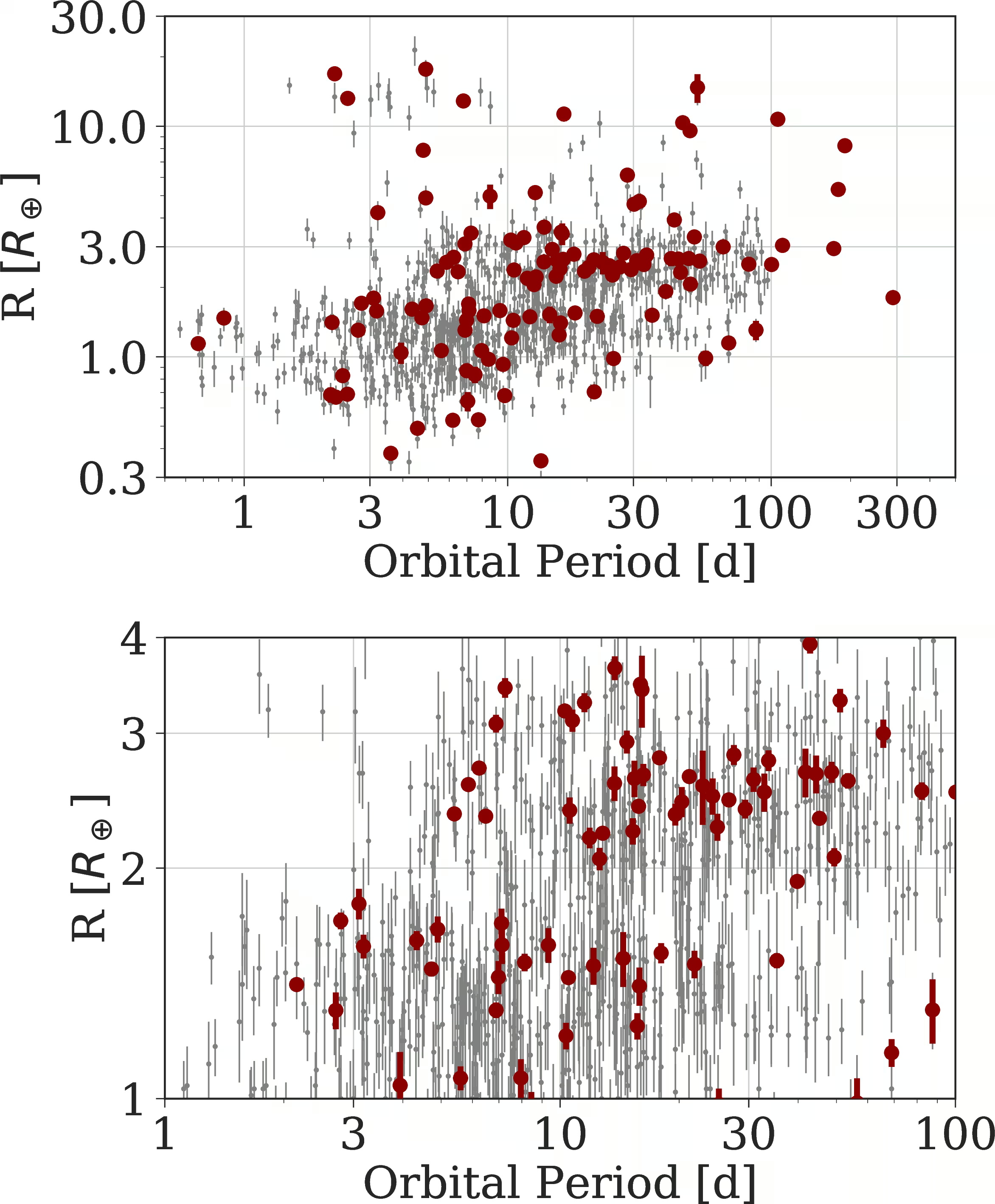
../_images/vaneylen_radius_valley.avif — Fig. 13.26 Slope of the **radius valley** with orbital period, from the asteroseismic Kepler subsample of Van Eylen *et al.* [2018]. The empirical valley boundary descends to smaller radii at longer periods, separating super-Earths from sub-Neptunes.#

Fig. 13.27 overlays the model predictions for the slope of the valley on these data.

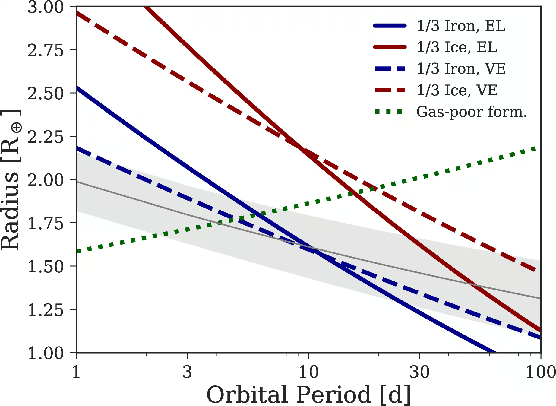
../_images/vaneylen_models.avif — Fig. 13.27 Model predictions for the slope of the radius valley with orbital period, overlaid on the Van Eylen *et al.* [2018] data. The black curves are different theoretical predictions; both photoevaporation and core-powered mass loss predict broadly compatible slopes, and the data alone cannot decisively prefer one over the other.#

Because stripping removes primordial envelopes, many close-in super-Earths are remnant cores rather than primordially rocky planets, although for any single planet the two origins cannot be told apart from bulk density alone.

13.4.4. The hot Neptune desert#

The hot Neptune desert is a deficit of Neptune-mass planets ($M_p \approx 10$ to $100\,\Mearth$) at orbital periods shorter than 5 days. While hot Jupiters and rocky planets occur at these periods, Mazeh et al. [2016] showed that hot Neptunes are absent (Fig. 13.28).

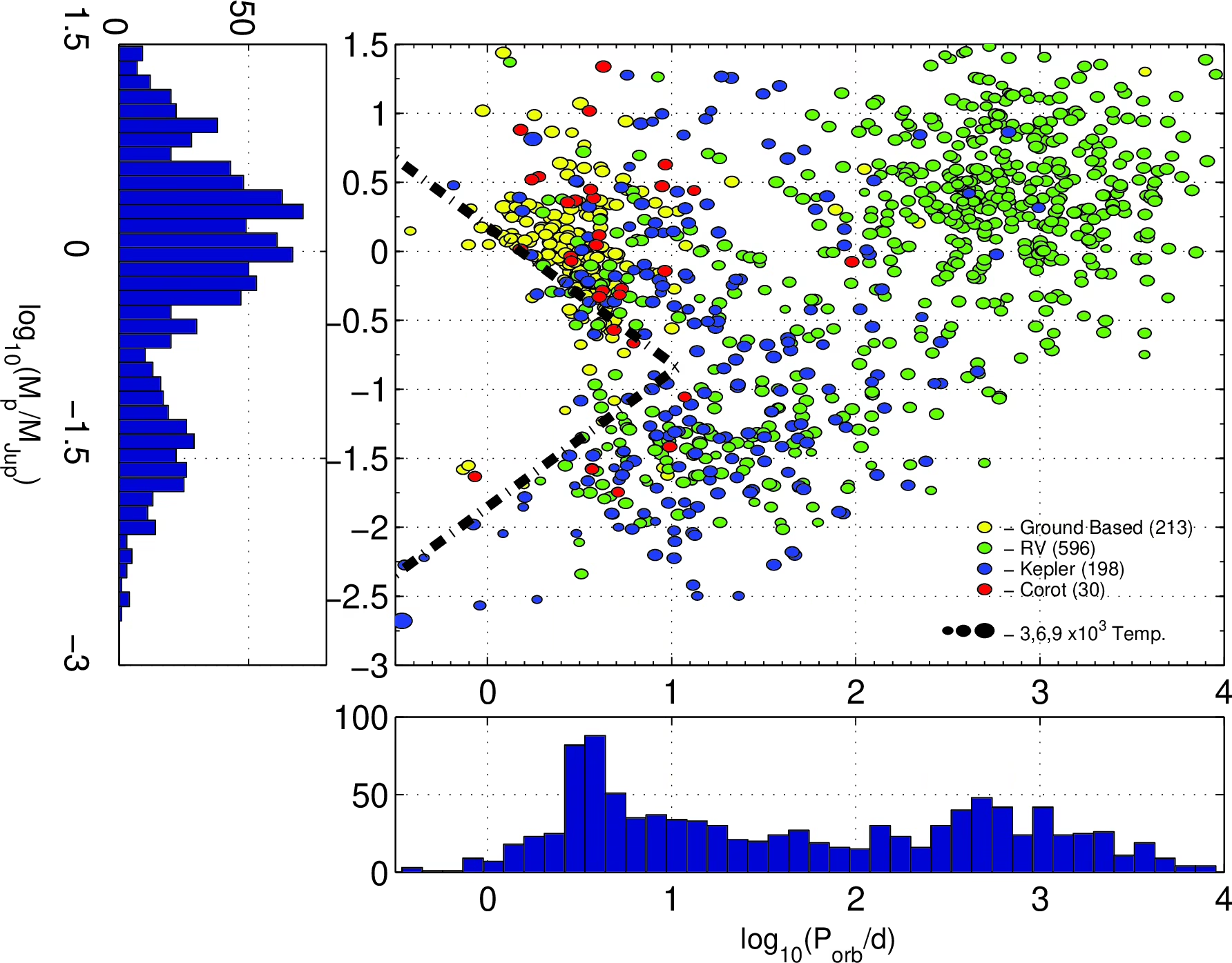
../_images/mazeh_neptune_desert.avif — Fig. 13.28 The **hot Neptune desert** in the period-mass and period-radius planes from Mazeh *et al.* [2016]. The shaded triangular region is empirically depleted of Neptune-mass planets. The upper edge follows a tight power law, plausibly set by Roche-lobe overflow on inflated hot Jupiters; the lower edge is more diffuse and has been variously attributed to photoevaporation, in-situ formation, and high-eccentricity migration with tidal circularization. The desert is one of the strongest pieces of evidence for atmospheric mass loss as a major sculptor of close-in planets.#

Photoevaporation strips envelopes from lower-mass planets below the desert, leaving bare super-Earths. At the upper edge, inflated planets fill their Roche lobe, the region where gas stays gravitationally bound to the planet rather than the star, losing mass through tidal stripping.

13.4.5. Planetary system architectures#

Multi-planet systems observed by Kepler enable statistical studies of planetary architecture. Weiss et al. [2018] identified a peas in a pod architecture, in which planets within the same system share similar sizes (Fig. 13.29) and regular orbital period spacing (Fig. 13.30).

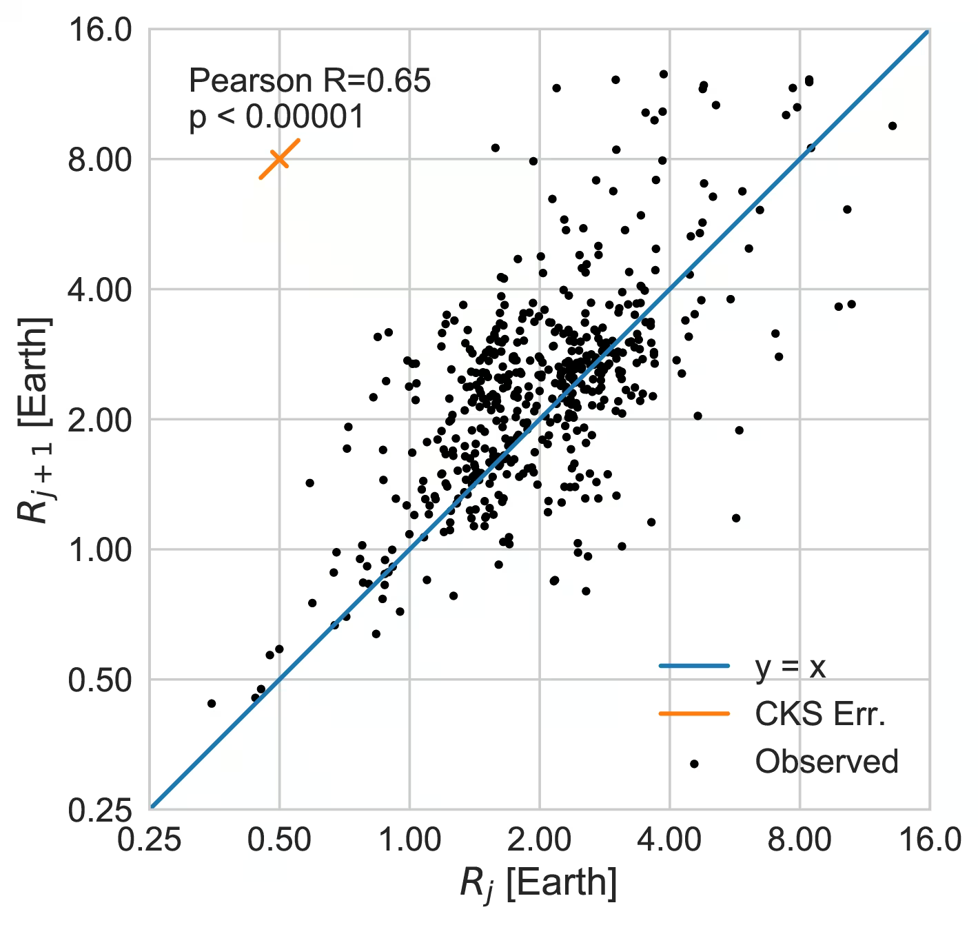
../_images/weiss_peas_in_pod.avif — Fig. 13.29 The **peas in a pod** correlation from Weiss *et al.* [2018]: the radius of an inner Kepler multi-planet $R_i$ versus the radius of its immediately outer neighbour $R_{i+1}$. The clear positive correlation along the diagonal means that within a system the planets tend to be the same size as each other, far more so than randomly drawn pairs of planets from the Kepler sample. The Pearson correlation coefficient is 0.65 and the null-hypothesis probability is $p < 10^{-7}$.#

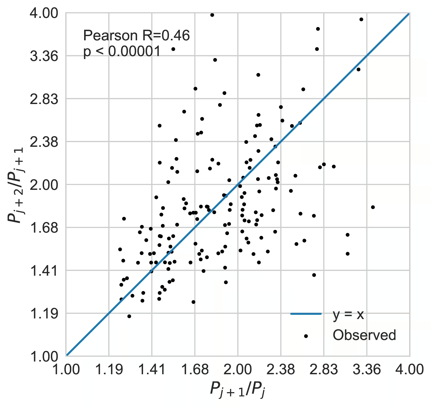
../_images/weiss_spacing.avif — Fig. 13.30 Period-ratio correlation in Kepler multi-planet systems, from Weiss *et al.* [2018]. Each point is a triple of consecutive transiting planets in the same system: the horizontal axis is the period ratio of the inner pair ($P_{j+1}/P_j$) and the vertical axis is the period ratio of the next pair out ($P_{j+2}/P_{j+1}$). The clustering along the diagonal (Pearson $R = 0.46$, $p < 10^{-5}$) means that within a system, neighbouring period ratios are similar, supporting the view that compact inner systems form by a smooth, local process rather than by stochastic large impacts.#

This regularity indicates that compact inner systems form through smooth growth and disk migration rather than stochastic giant impacts. In contrast, terrestrial planet assembly in the solar system was dominated by giant impacts (Lecture 2), suggesting the inner solar system may be dynamically unusual.

This pattern is a statistical trend for compact systems rather than a universal rule. Radial-velocity samples of wider systems and exceptional Kepler architectures exhibit greater diversity.

Resonant chains provide direct evidence that early disk migration locked planets into place before gas dispersal. For example, TRAPPIST-1 contains seven Earth-sized planets in mean-motion resonances within 0.06 AU [Gillon et al., 2017].

13.4.6. Hot Jupiters and migration#

The inner edge of the surviving population is set by the fluid Roche limit, the orbital separation where stellar tides tear a planet apart:

\[ d_R \approx 2.46\,R_\star \left(\frac{\rho_\star}{\rho_p}\right)^{1/3}. \]

For a Sun-like star ($\rho_\star \approx 1.4$ g cm$^{-3}$) and a hot Jupiter ($\rho_p \approx 1$ g cm$^{-3}$), this limit gives $d_R \approx 2.7\,R_\star \approx 0.013$ AU. The observed pile-up of hot Jupiters at $\sim 0.04$ to $0.05$ AU sits a factor of three to four outside this limit, where orbits survive over Gyr timescales without tidal disruption.

In disk migration (Type II), net torques in a gaseous disk drive inward migration (Lecture 2), preserving low eccentricities and alignment with the stellar equator.

In high-eccentricity migration, Kozai-Lidov oscillations over $10^{6}$ to $10^{8}$ years drive perihelion near the star, where tidal dissipation circularises the orbit while freezing in large misalignments.

In planet-planet scattering, dynamical instabilities in multi-giant systems eject planets and leave misaligned survivors circularised by tides (Fig. 13.31).

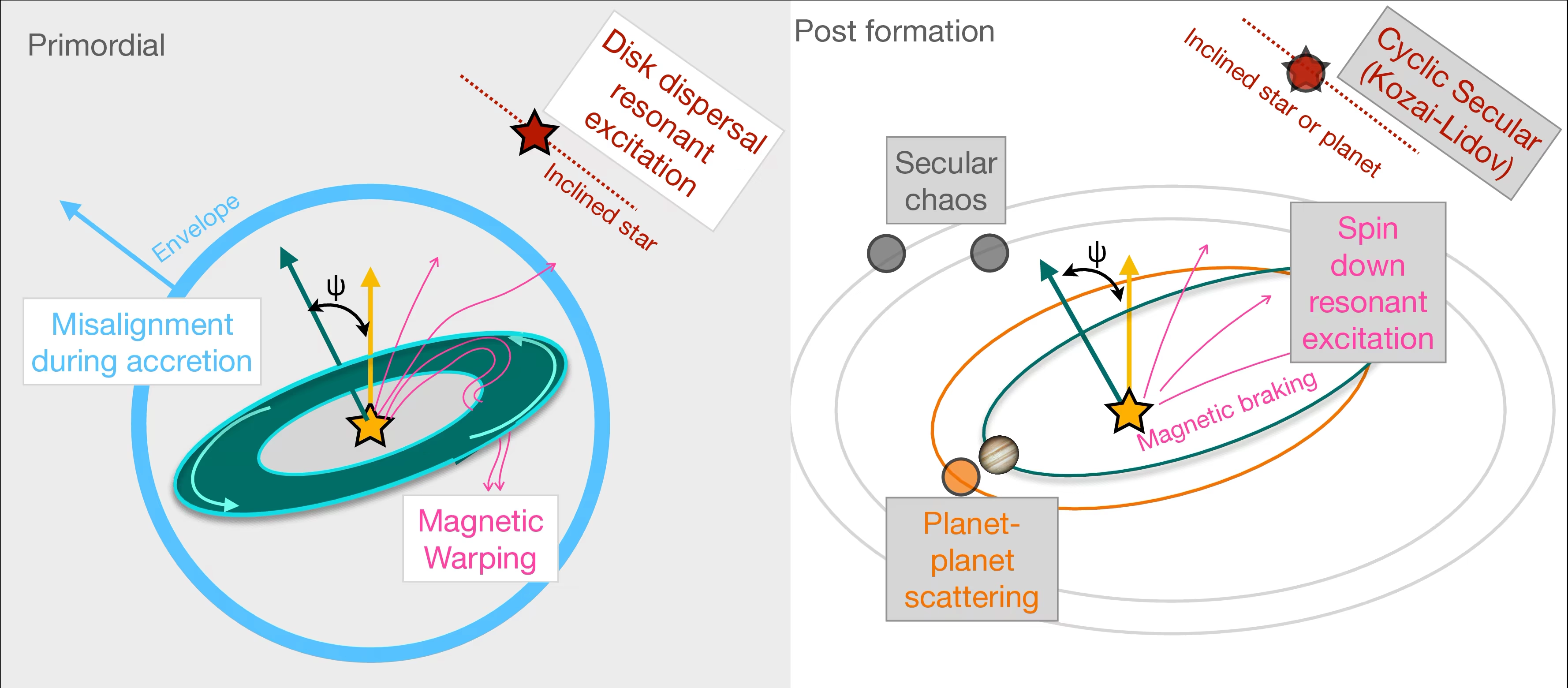
../_images/obliquity_pathways.avif — Fig. 13.31 Schematic of the three migration pathways for hot Jupiters and the **stellar obliquities** they produce, from the review of Albrecht *et al.* [2022]. Disk migration preserves spin-orbit alignment, whereas high-eccentricity migration and planet-planet scattering produce large misalignments.#

These pathways are distinguished observationally by the stellar obliquity (spin-orbit angle), measured via the Rossiter-McLaughlin effect (Fig. 13.32) as a transiting planet sequentially occults the blueshifted and redshifted stellar hemispheres. Hiding blueshifted light makes the remaining starlight appear redshifted, and the reverse, so the measured radial velocity shows an anomaly of order $(R_p/R_\star)^2\, v \sin i_\star$ during the transit, where $v \sin i_\star$ is the projected rotation velocity of the star; for a hot Jupiter this is tens of m/s. An aligned orbit gives an anomaly that is antisymmetric about mid-transit, a misaligned orbit an asymmetric one, and a retrograde orbit reverses its sign. The effect measures the sky-projected obliquity $\lambda$, the angle between the projected stellar spin axis and the orbit normal; the orbital inclination $i$ comes from the transit light curve. Hot Jupiters around cool stars ($T_\mathrm{eff} < 6250$ K) are mostly well aligned, reflecting disk migration or tidal realignment in convective envelopes. Hot Jupiters around hot stars ($T_\mathrm{eff} > 6250$ K) show wide misalignments spanning prograde to retrograde orbits [Albrecht et al., 2022] (Fig. 13.33).

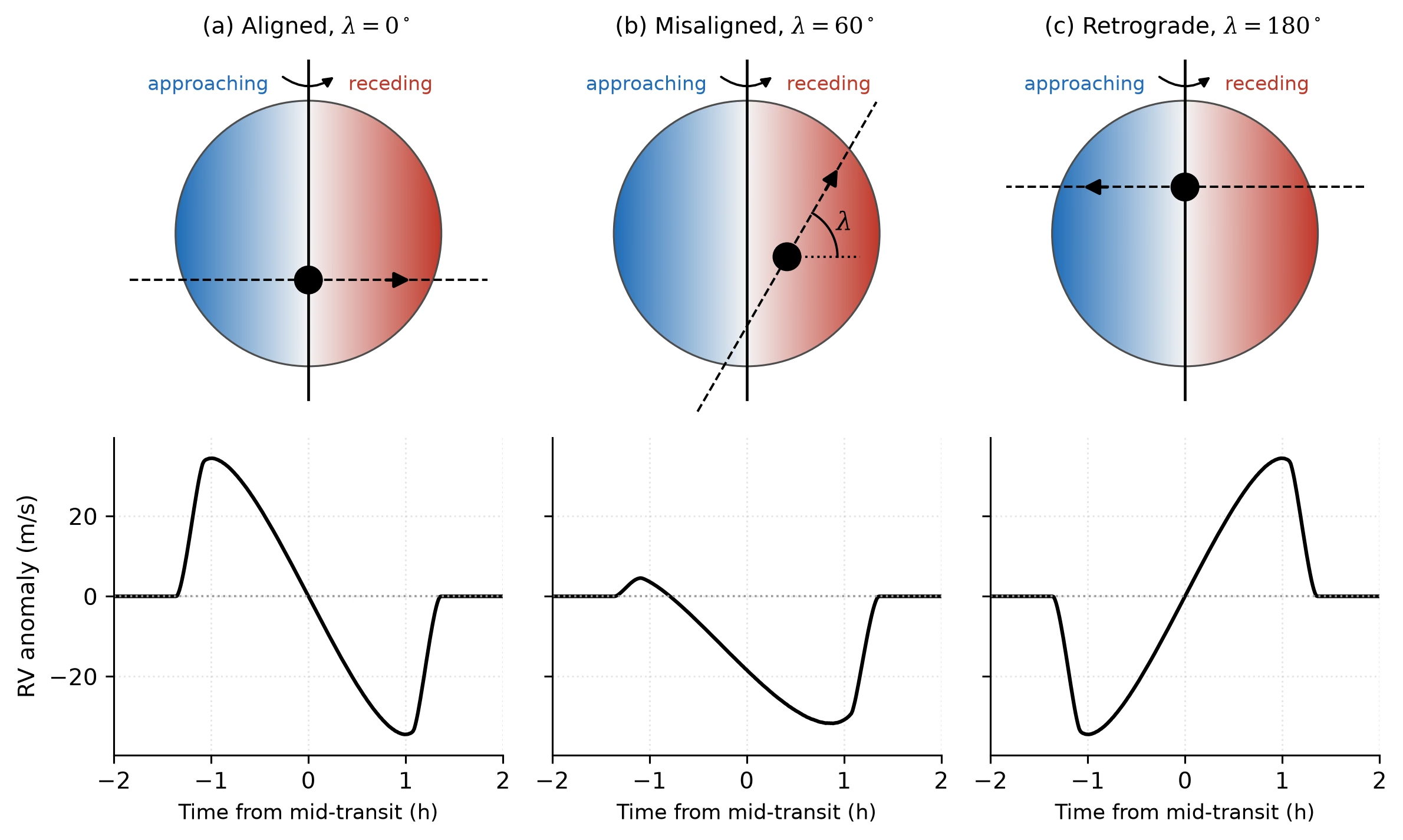
../_images/rossiter_mclaughlin_obliquity.avif — Fig. 13.32 The **Rossiter-McLaughlin effect** for a hot Jupiter ($R_p/R_\star = 0.1$, impact parameter $0.35$) crossing a Sun-like star with projected rotation velocity $v \sin i_\star = 5$ km s$^{-1}$. Top: the stellar disk coloured by line-of-sight velocity (blue approaching, red receding), the projected spin axis (vertical line) and the transit chord (dashed, arrow in the direction of motion). Bottom: the radial velocity anomaly during the transit. (a) Aligned orbit, $\lambda = 0^\circ$: the planet first hides approaching light, the remaining light appears redshifted, and the anomaly is antisymmetric. (b) Misaligned orbit, $\lambda = 60^\circ$: the chord crosses mainly the receding half and the anomaly is asymmetric. (c) Retrograde orbit, $\lambda = 180^\circ$: the anomaly has the opposite sign. The shape of the anomaly gives the sky-projected obliquity $\lambda$; the orbital inclination comes from the transit light curve. First-moment model on a pixel grid with linear limb darkening ($u = 0.6$). Course-original figure.#

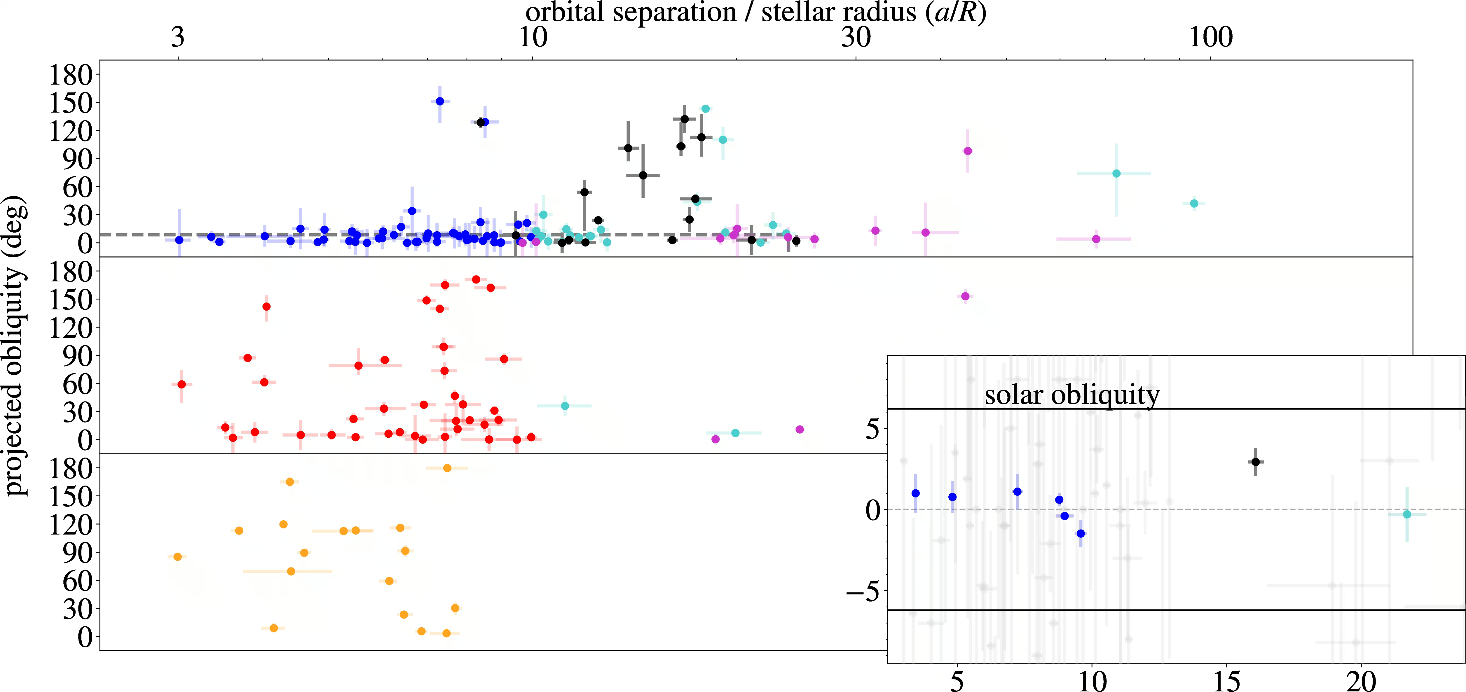
../_images/obliquity_distribution.avif — Fig. 13.33 Projected stellar obliquity $\lambda$ as a function of scaled orbital separation $a/R_\star$ for the hot Jupiter sample, from Albrecht *et al.* [2022]. Tight orbits around cool stars cluster near zero obliquity from tidal realignment, whereas wider scatter around hotter hosts indicates a wide primordial obliquity distribution.#

13.4.7. Super-Earth and sub-Neptune composition#

Bulk-density measurements combining transit and radial-velocity data enable a compositional census of small planets. Super-Earths below the radius valley have rocky compositions with densities of $4$ to $8$ g/cm$^3$, similar to Earth and Venus. Sub-Neptunes above the valley have lower densities, typically $1$ to $3$ g/cm$^3$, requiring a volatile envelope of $\mathrm{H_2}$/He or $\mathrm{H_2O}$ over a rocky core. Bulk density alone is degenerate: multiple internal structures can match the same bulk density, as shown by comparing observed planet masses and radii against theoretical composition curves (Fig. 13.34).

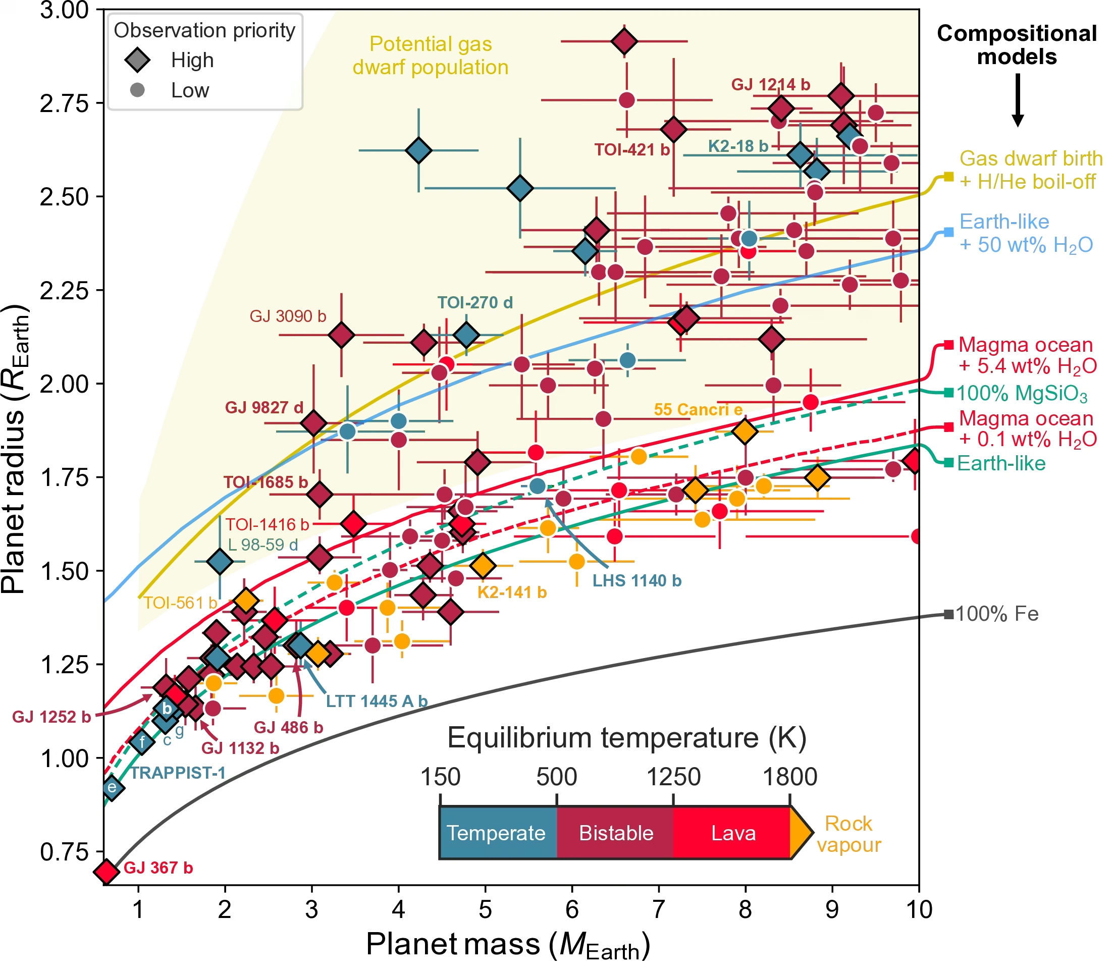
../_images/lichtenberg2025_mass_radius.avif — Fig. 13.34 Mass-radius distribution of small exoplanets compared with theoretical interior models ranging from pure iron to volatile-rich envelopes, categorized by thermal regime. Rocky super-Earths align closely with silicate-iron curves, whereas sub-Neptunes require substantial volatile envelopes or water-rich layers to explain their larger radii. Reproduced from Lichtenberg *et al.* [2025].#

Sub-Neptunes with $\gtrsim 10$ to $20\%$ $\mathrm{H_2O}$ by mass are candidate water worlds. In the proposed hycean scenario, a planet hosts a shallow liquid water ocean beneath a thick $\mathrm{H_2}$-rich atmosphere [Madhusudhan et al., 2021]. The strong $\mathrm{H_2}$ greenhouse effect can keep the ocean liquid at equilibrium temperatures below 273 K, extending the candidate habitable region. This interpretation is contested: observations of K2-18 b may reflect mini-Neptunes without a surface, or an $\mathrm{H_2}$ envelope over a deep magma ocean [Shorttle et al., 2024].

13.4.8. M dwarf planets#

M dwarfs account for roughly 75% of main-sequence stars and are the easiest targets for discovering small habitable-zone planets. Because the habitable-zone semi-major axis scales as $\sqrt{L_\star}$, closer orbits around low-luminosity M dwarfs increase the geometric transit probability $R_\star / a$. The transit depth $(R_p / R_\star)^2$ for an Earth-sized planet is also much larger than around a Sun-like star.

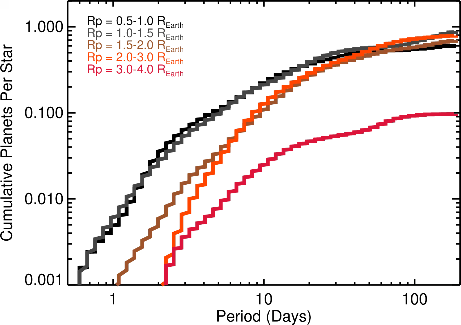
../_images/dressing_mdwarf_occurrence.avif — Fig. 13.35 Cumulative occurrence rate of small planets around M dwarfs as a function of orbital period from the full Kepler sample, from Dressing and Charbonneau [2015]. Each curve is a different planet-radius bin from $0.5$–$1\,\Rearth$ (black) to $3$–$4\,\Rearth$ (red). M dwarfs host on average $\sim 2$ small planets per star inside 200 days, and roughly one Earth-size planet per star in or near the habitable zone. M dwarf small-planet occurrence rates exceed those around Sun-like stars by roughly a factor of 2–3.#

Kepler occurrence rates indicate roughly $2.5$ small planets ($R_p < 4\,\Rearth$) per M dwarf inside 200 days, with $0.16^{+0.17}_{-0.07}$ Earth-size planets in the conservative habitable zone (Fig. 13.35) [Dressing and Charbonneau, 2015].

The main challenge for habitability is stellar activity, the elevated magnetic and high-energy emission of the host star. M dwarfs spend hundreds of Myr in an early phase with luminosities up to ten times their main-sequence values. Habitable-zone planets sit inside their runaway-greenhouse boundary during this phase, causing severe water loss. High XUV flux can strip an Earth-equivalent ocean of water, leaving an abiotic oxygen atmosphere as a false-positive biosignature (a chemical sign mimicking life) [Luger and Barnes, 2015].

A second challenge is tidal locking, the synchronization of rotation and orbit into a $1{:}1$ spin-orbit resonance. Close-in orbits produce permanent daysides and nightsides, requiring atmospheric heat transport to prevent volatile collapse on the nightside. Three-dimensional climate models show that substellar clouds can stabilize climates and extend the habitable zone closer to the star [Yang et al., 2013]. The seven planets of TRAPPIST-1 are a primary laboratory to study these climate regimes.

13.5. Part 3: Characterisation, habitability, and the comparative payoff#

13.5.1. Transmission spectroscopy during transit#

During transit, atmospheric absorption along the terminator sets the wavelength-dependent transit depth:

\[ \delta(\lambda) = \frac{[R_p + n_H H(\lambda)]^2}{R_\star^2}, \]

where $H = \kB T / (\mu m_u g)$ is the atmospheric scale height (the density e-folding scale, derived in Lecture 5). For a hot Jupiter ($T \approx 1500$ K, $\mu \approx 2.3$, $g \approx 25$ m s$^{-2}$):

\[ H = \frac{\kB T}{\mu m_u g} = \frac{(1.38 \times 10^{-23})(1500)}{(2.3)(1.66 \times 10^{-27})(25)} \approx 2 \times 10^{5}\ \mathrm{m}, \]

With $R_p \approx 1.2\,\Rjup$, $R_\star \approx 1\,\Rsun$, and $n_H \approx 5$:

\[ \frac{\Delta\delta}{\delta} \approx \frac{2 n_H H}{R_p} \approx \frac{2 \times 5 \times 2 \times 10^{5}\ \mathrm{m}}{8.6 \times 10^{7}\ \mathrm{m}} \approx 2 \times 10^{-2}, \]

The absolute depth change $(\Delta\delta / \delta) \times \delta \approx 2 \times 10^{-4}$ (a few hundred ppm) is detectable with JWST. Sub-Neptunes reach 10 to 100 ppm, while terrestrial planets around M dwarfs fall below 10 ppm.

High-altitude clouds and hazes flatten transmission spectra via continuum opacity, spanning from clear to cloudy atmospheres (Sing et al. [2016], Fig. 13.36; Fig. 13.37).

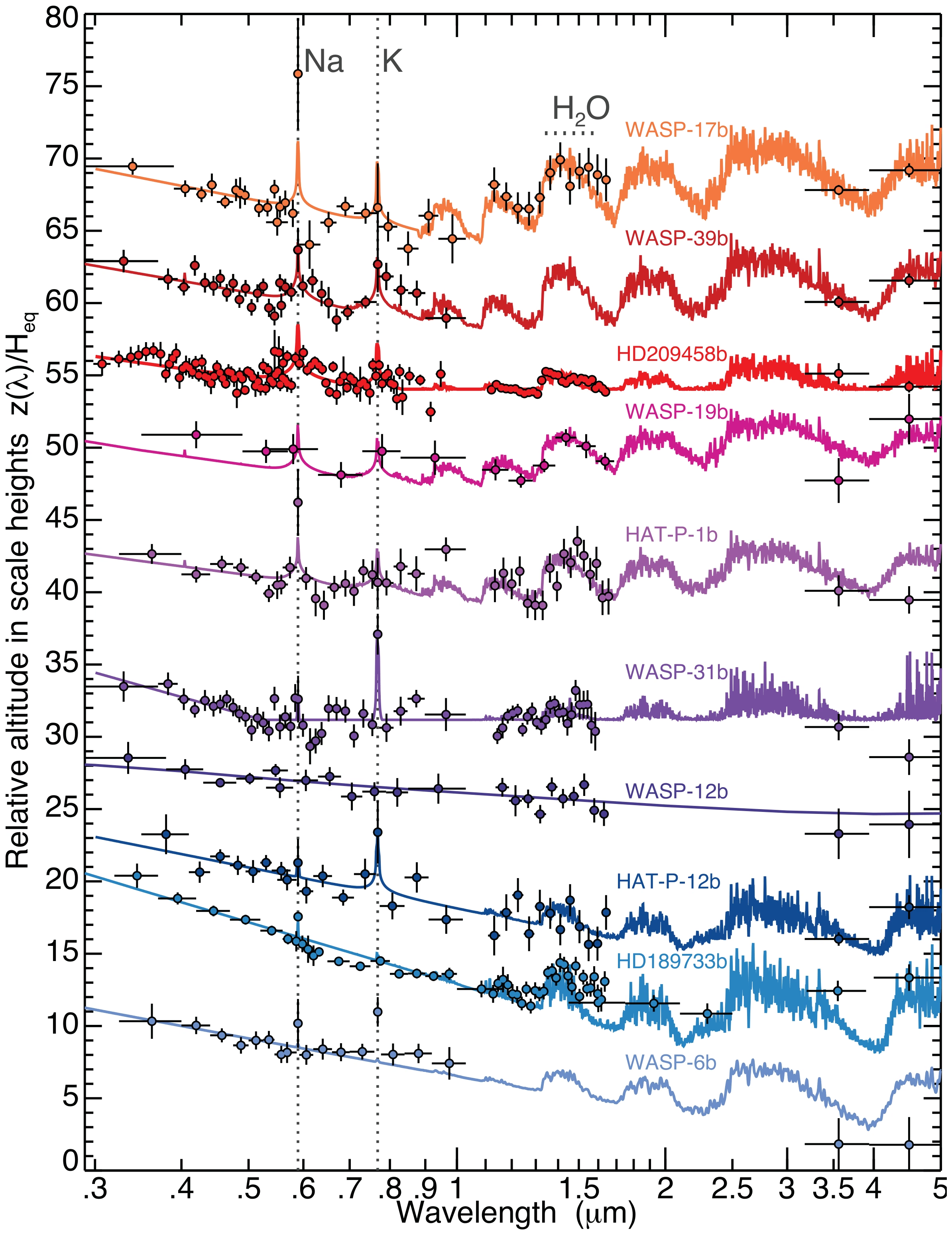
../_images/sing_hotjup_spectra.avif — Fig. 13.36 Transmission spectra of ten hot Jupiters observed with HST and Spitzer across wavelengths from $0.3$ to $5$ $\mu$m on a logarithmic scale, plotted as relative altitude $z(\lambda)/H_{\rm eq}$ with $1\sigma$ uncertainties and offset vertically, from Figure 1 of Sing *et al.* [2016]. Spectra are ordered from top to bottom by increasing altitude difference $\Delta Z_{\rm UB-LM}$ between the blue-optical and mid-infrared, showing a continuum from clear atmospheres with Na and K resonance lines ($0.59$ and $0.77$ $\mu$m) and $\mathrm{H_2O}$ absorption ($1.4$ $\mu$m) in WASP-17 b to aerosol-dominated scattering slopes in WASP-6 b.#

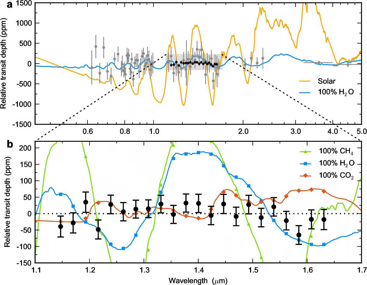
../_images/gj1214b_clouds.avif — Fig. 13.37 Featureless transmission spectrum of the warm sub-Neptune **GJ 1214 b** from Kreidberg *et al.* [2014], showing how high-altitude clouds or hazes erase atmospheric absorption features in high-precision HST data. Three cloud-free model atmospheres ($\mathrm{H_2O}$, $\mathrm{CH_4}$, $\mathrm{CO_2}$) are ruled out at high significance, demonstrating that the flat spectrum requires an optically thick cloud or haze layer at high altitude.#

13.5.2. Emission spectroscopy and phase curves#

Emission spectroscopy observes planetary thermal radiation during secondary eclipse, when the planet passes behind the star. The flux drop yields the dayside brightness temperature, the equivalent blackbody temperature. A phase curve tracks orbital brightness, where day-night contrast reveals heat redistribution efficiency (Fig. 13.38).

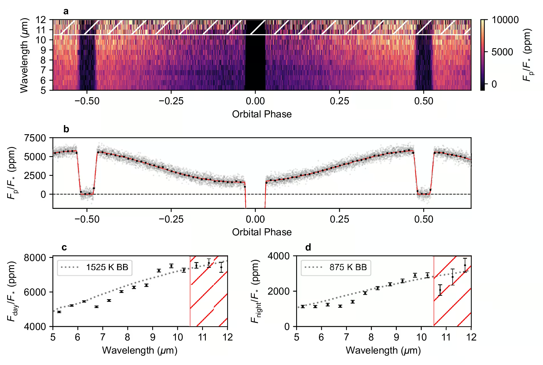
../_images/wasp43b_phase_curve.avif — Fig. 13.38 JWST MIRI **phase curve** of the hot Jupiter **WASP-43 b**, from Bell *et al.* [2024]. The top panel is the spectroscopic phase curve as a function of wavelength and orbital phase. The middle panel is the band-integrated white light curve, showing one transit, two secondary eclipses, and the smooth phase modulation of the planet’s thermal flux as the dayside rotates in and out of view. The bottom panels are the dayside and nightside emission spectra and best-fit blackbody models. The retrieved nightside temperature is much colder than the dayside, evidence of a strong day-night contrast despite an atmosphere thick enough to imprint clear spectral features on the dayside.#

Combining transmission, emission, and phase curves constrains atmospheric thermal structure, composition, and circulation.

13.5.3. JWST era results (2022–2025)#

The James Webb Space Telescope has transformed exoplanet atmospheric characterisation since mid-2022. Transmission spectroscopy of the hot Saturn WASP-39 b revealed $\mathrm{H_2O}$, $\mathrm{CO_2}$, Na, and CO, while the absence of $\mathrm{CH_4}$ indicates super-solar metallicity [Alderson et al., 2023, Rustamkulov et al., 2023] (Fig. 13.39) (Fig. 13.41).

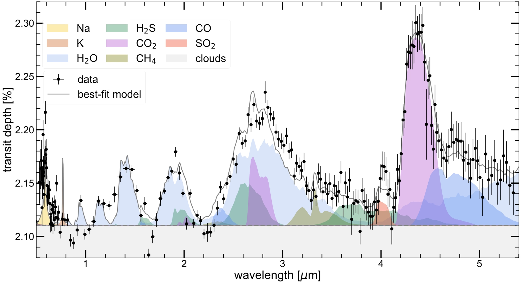
../_images/wasp39b_prism_spectrum.avif — Fig. 13.39 The JWST/NIRSpec PRISM transmission spectrum of **WASP-39 b**, from Figure 4 of Rustamkulov *et al.* [2023], plots measured transit depths in per cent with $1\sigma$ uncertainties from $0.5$ to $5.5\ \mu\mathrm{m}$ against the best-fitting PICASO 3.0 grid model with shaded species opacity contributions. The data confirm clear detections of $\mathrm{H_2O}$ ($33\sigma$, $1$–$2.2\ \mu\mathrm{m}$), $\mathrm{CO_2}$ ($28\sigma$, $4.3\ \mu\mathrm{m}$), a flat grey cloud deck ($21\sigma$), Na ($19\sigma$, $0.58\ \mu\mathrm{m}$), and CO ($7\sigma$, $4.7\ \mu\mathrm{m}$), whereas K, $\mathrm{H_2S}$, and $\mathrm{CH_4}$ model contributions are not favoured despite detector saturation between $0.8$ and $1.9\ \mu\mathrm{m}$.#

The detection of $4$ $\mu$m absorption from $\mathrm{SO_2}$ is the first identification of a photochemical product, a molecule generated by stellar irradiation rather than thermochemical equilibrium, in an exoplanet atmosphere [Tsai et al., 2023] (Fig. 13.40). The signal is modest in each instrument ($2.7\sigma$ to $4.8\sigma$), and the case rests on two instruments seeing the same feature and on four photochemistry codes reproducing it. Its formation requires ultraviolet photolysis of $\mathrm{H_2S}$ followed by oxidation of sulfur to SO and $\mathrm{SO_2}$.

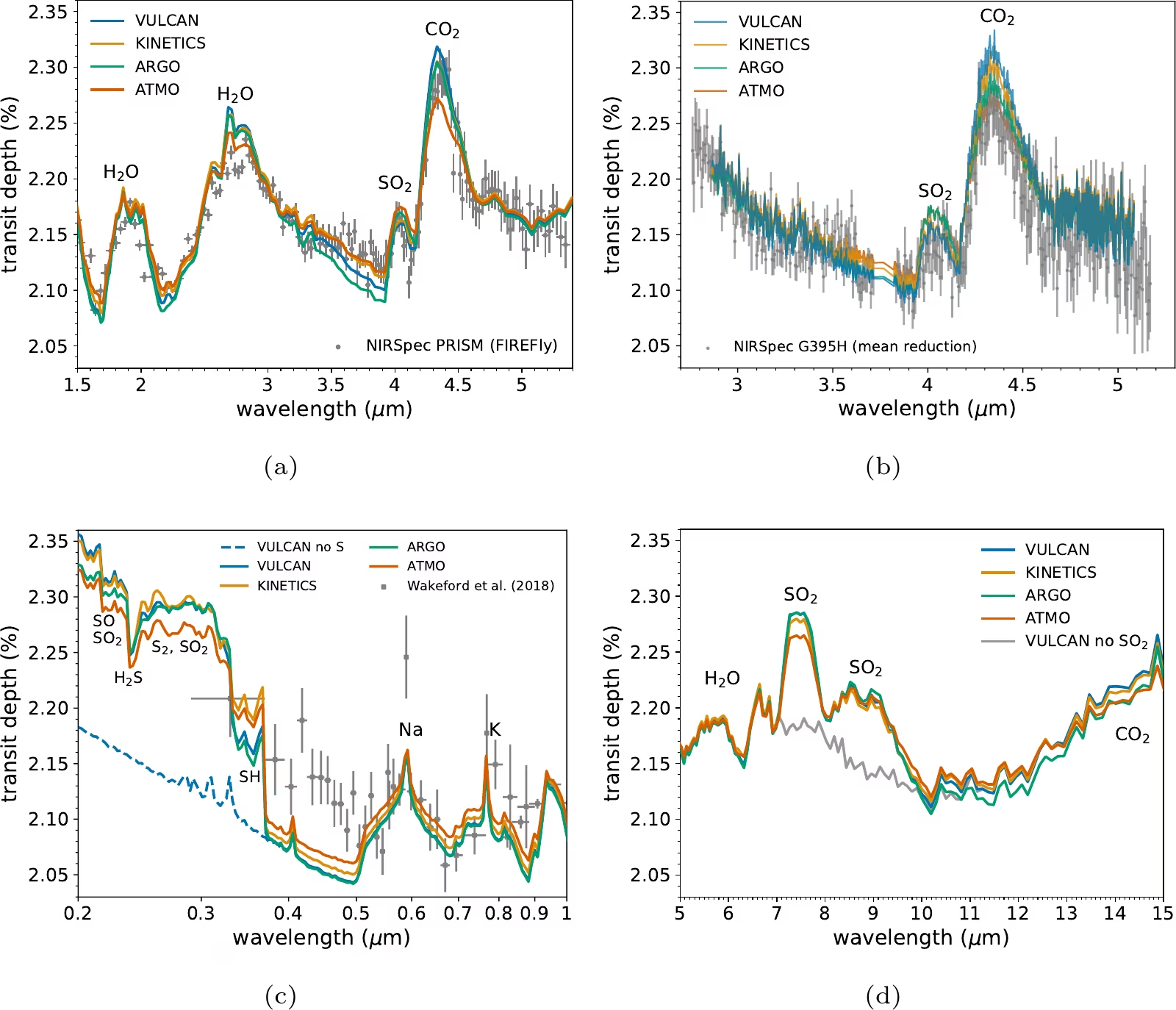
../_images/wasp39b_so2_spectrum.avif — Fig. 13.40 Terminator-averaged theoretical transmission spectra of WASP-39 b from photochemical models comparing four codes (VULCAN, KINETICS, ARGO, ATMO) against NIRSpec PRISM, NIRSpec G395H, and optical HST and VLT/FORS2 data, from Figure 3 of Tsai *et al.* [2023]. All four independent codes reproduce the observed $4.05\ \mu\mathrm{m}$ $\mathrm{SO_2}$ feature, confirming the role of sulfur photochemistry in atmospheric opacity, and predict stronger bands across the $5$–$15\ \mu\mathrm{m}$ MIRI range near $7.5$ and $8.7\ \mu\mathrm{m}$.#

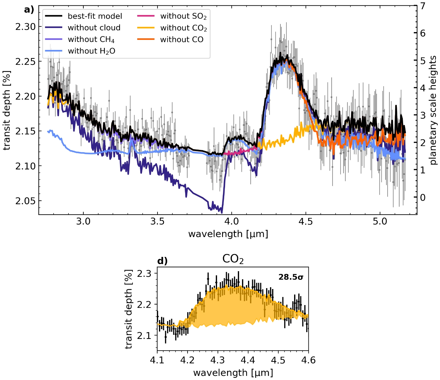
../_images/wasp39b_alderson_species.avif — Fig. 13.41 Contribution of individual opacity sources to the JWST/NIRSpec G395H transmission spectrum of WASP-39 b, from Figure 4 of Alderson *et al.* [2023]. Panel a is the full spectrum. Grey points with error bars are the measurement, the black curve is the best-fitting model with an injected $\mathrm{SO_2}$ volume mixing ratio of $10^{-5.6}$, and each coloured curve is that same model with one opacity source removed: cloud, $\mathrm{CH_4}$, $\mathrm{H_2O}$, $\mathrm{SO_2}$, $\mathrm{CO_2}$, or CO. The left axis is transit depth in per cent and the right axis is the same quantity in planetary scale heights; the horizontal axis is wavelength in $\mu$m. The wavelength range where a coloured curve separates from the black one is the range in which that species absorbs. Panel d is the $\mathrm{CO_2}$ band near 4.3 $\mu$m on its own: black points are the measurement and the shaded orange region is the difference that the $\mathrm{CO_2}$ opacity makes to the model. The band is detected at $28.5\sigma$, above the $21.5\sigma$ of $\mathrm{H_2O}$ and the $4.8\sigma$ of $\mathrm{SO_2}$ in the same spectrum.#

For TRAPPIST-1 b, $15\ \mu\mathrm{m}$ thermal emission is consistent with a bare rock dayside in radiative equilibrium with no atmospheric heat redistribution, ruling out a thick $\mathrm{CO_2}$ atmosphere [Greene et al., 2023]; the same measurement for TRAPPIST-1 c [Zieba et al., 2023] rules out a thick Venus-like atmosphere and suggests that the innermost rocky planets of active M dwarfs are stripped (Lecture 5) (Fig. 13.42, Fig. 13.43).

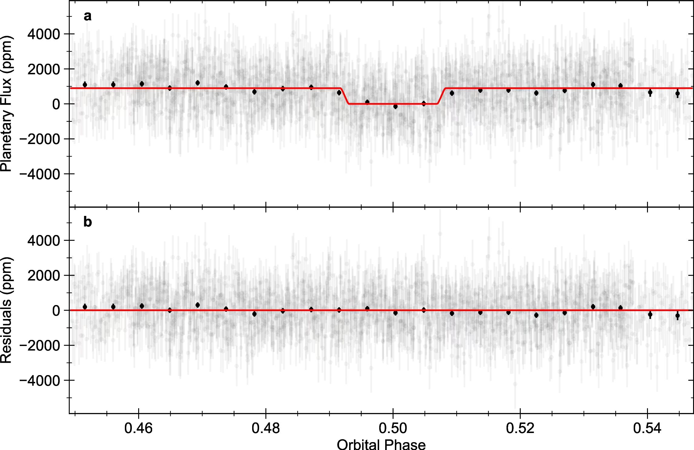
../_images/trappist1b_eclipse.avif — Fig. 13.42 JWST MIRI $15\ \mu\mathrm{m}$ secondary eclipse light curve of **TRAPPIST-1 b** from Greene *et al.* [2023], marking the first thermal emission detection of an Earth-sized exoplanet. The eclipse depth $f_p / f_\star = 861 \pm 99$ ppm corresponds to a dayside brightness temperature of $T_B = 503^{+26}_{-27}$ K, matching the $508$ K bare-rock prediction in radiative equilibrium with no significant heat redistribution.#

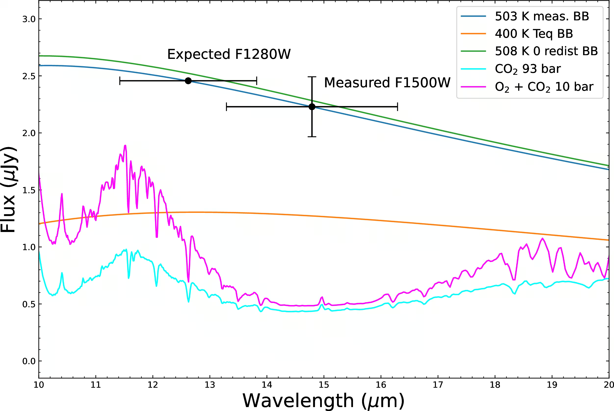
../_images/trappist1b_emission.avif — Fig. 13.43 The TRAPPIST-1 b dayside emission compared with model atmospheres of different compositions, from Greene *et al.* [2023]. The data are inconsistent with thick $\mathrm{CO_2}$ + $\mathrm{N_2}$ atmospheres and inconsistent with $\mathrm{O_2}$ + $\mathrm{CO_2}$ atmospheres at any plausible mass-loading. They are consistent with a bare-rock dayside (the 503 K blackbody curve, magenta).#

Secondary eclipse observations of the hot rocky super-Earth 55 Cancri e by Hu et al. [2024] show a dayside cooler than expected for bare rock (Fig. 13.44). This provides tentative evidence for a secondary atmosphere, a volatile envelope outgassed from a molten surface.

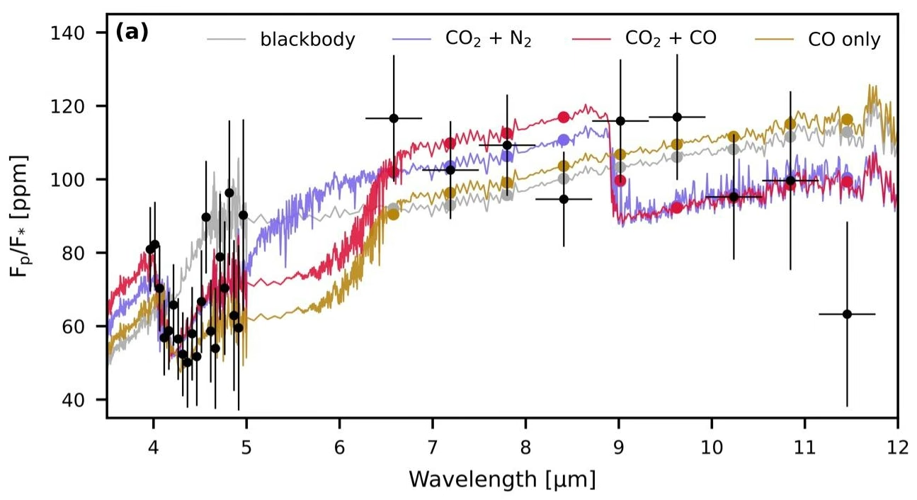
../_images/55cnce_hu_emission.avif — Fig. 13.44 JWST/NIRCam plus MIRI thermal emission spectrum of **55 Cancri e** from Hu *et al.* [2024]. Black points are the binned JWST data; coloured curves are atmospheric models (grey blackbody, $\mathrm{CO_2}$+$\mathrm{N_2}$ purple, $\mathrm{CO_2}$+CO red, CO-only gold). The data fall below the bare-rock blackbody at most wavelengths and favour atmospheric models with non-negligible CO and $\mathrm{CO_2}$. A companion retrieval (not shown) constrains the volatile mixing ratios but is sensitive to the assumed background gas, so the conclusion of a secondary atmosphere is currently tentative but suggestive.#

Flat transmission spectra for LHS 475 b [Lustig-Yaeger et al., 2023] and GJ 1132 b further indicate that small rocky M dwarf planets generally lose their atmospheres to early stellar activity (Fig. 13.45). A tentative water signal on GJ 486 b remains ambiguous due to stellar starspots [Moran et al., 2023].

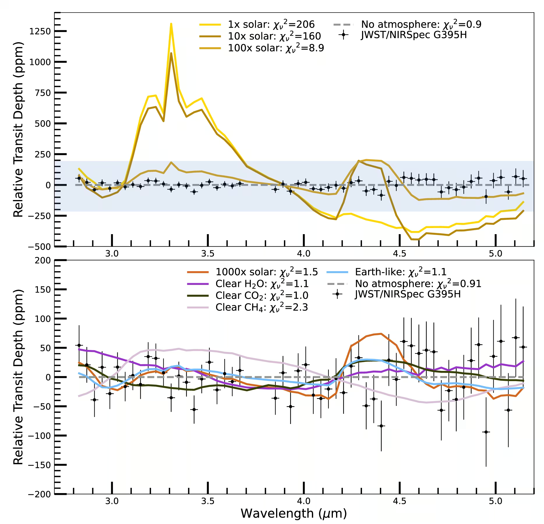
../_images/lhs475b_spectrum.avif — Fig. 13.45 JWST/NIRSpec G395H transmission spectrum of the rocky exoplanet **LHS 475 b**, an Earth-size M dwarf planet at $\sim 12$ pc, from Lustig-Yaeger *et al.* [2023]. The data are flat and featureless. Hydrogen-helium-dominated atmospheres are ruled out at high confidence (top panel). A pure $\mathrm{CH_4}$ atmosphere is also ruled out, though a pure $\mathrm{CO_2}$ Venus-like atmosphere is marginally consistent (bottom panel). The result is consistent with no detectable atmosphere on LHS 475 b.#

The habitable-zone sub-Neptune K2-18 b exhibits $\mathrm{CH_4}$ and $\mathrm{CO_2}$ alongside a marginal $2\sigma$ detection of dimethyl sulfide (DMS), initially interpreted as evidence for a hycean world with a liquid-water ocean [Madhusudhan et al., 2023] (Fig. 13.46).

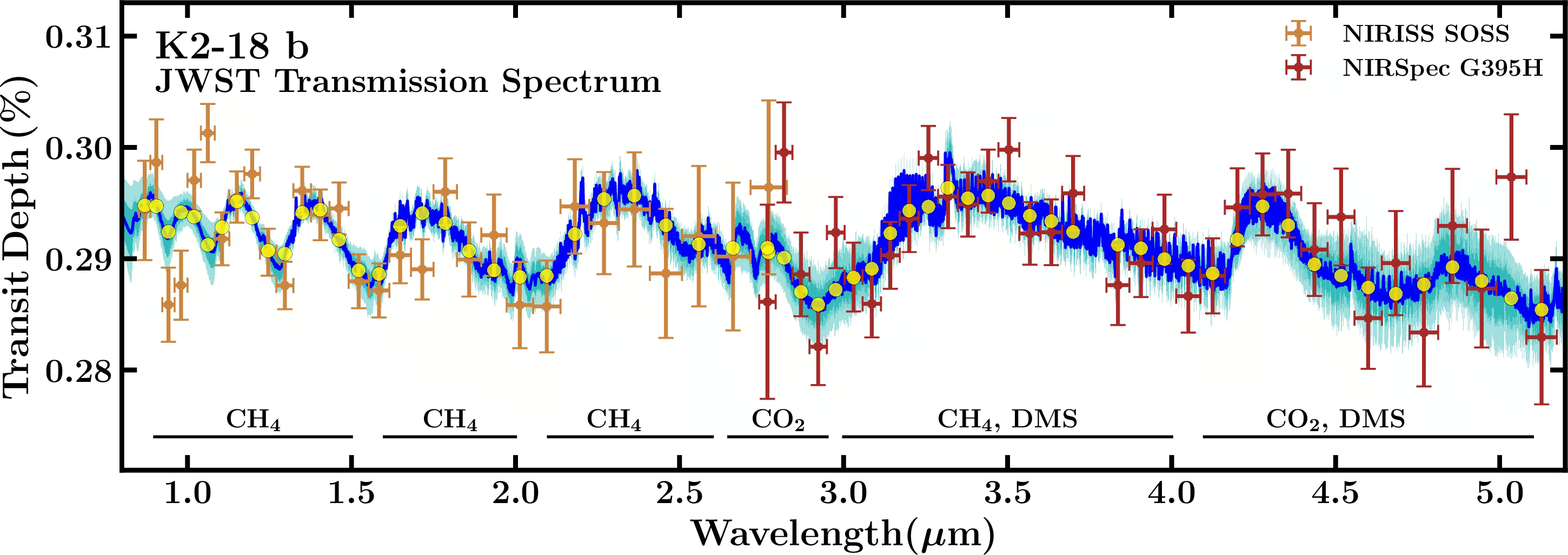
../_images/k218b_spectrum.avif — Fig. 13.46 JWST transmission spectrum of **K2-18 b** from Madhusudhan *et al.* [2023], combining NIRISS SOSS and NIRSpec G395H observations with colour-coded model spectra containing $\mathrm{CH_4}$, $\mathrm{CO_2}$, and tentatively dimethyl sulfide (DMS). While the $\mathrm{CH_4}$ and $\mathrm{CO_2}$ detections are clear, the tentative DMS feature lies near the JWST sensitivity floor and remains heavily dependent on retrieval assumptions.#

Subsequent reanalyses disputed the DMS detection, showing the data are also consistent with an uninhabitable mini-Neptune [Wogan et al., 2024], with an interior too hot to hold a liquid water ocean [Glein, 2024], or with an atmosphere overlying a magma ocean, a molten interior that depletes $\mathrm{NH_3}$ by dissolving nitrogen [Shorttle et al., 2024]. Like past debates over Martian methane (Lecture 10) and Venusian phosphine (Lecture 14), K2-18 b illustrates how tentative biosignature claims undergo community scrutiny and revision.

13.5.4. The habitable zone revisited#

The classical habitable zone is the range of stellar fluxes where a rocky planet can maintain liquid surface water (Lecture 9). Kasting et al. [1993] identified two boundaries using a one-dimensional radiative-convective model. The inner edge is set by the runaway greenhouse limit: rising water vapour caps outgoing longwave radiation at $280$ to $310$ W/m$^2$, evaporating the ocean. For a Sun-like star, this occurs at $\sim 1.06$ times Earth’s flux ($\sim 0.97$ AU), with the conservative moist greenhouse limit at $\sim 0.99$ AU. The outer edge is set by the maximum $\mathrm{CO_2}$ greenhouse. Adding $\mathrm{CO_2}$ first lowers the outgoing infrared flux, but near $10$ bar the atmosphere becomes optically thick at all infrared wavelengths and the outgoing flux stops falling, while Rayleigh scattering by $\mathrm{CO_2}$ continues to raise the planetary albedo; condensation of $\mathrm{CO_2}$ also lowers the tropospheric lapse rate and weakens the greenhouse effect. Beyond the point where the albedo increase outweighs the extra greenhouse warming, more $\mathrm{CO_2}$ cools the planet [Kopparapu et al., 2013]. For the present Sun this limit lies at $S_{\mathrm{eff}} \approx 0.35\,S_\oplus$, or $\sim 1.69$ AU.

This one-dimensional limit leaves out $\mathrm{CO_2}$ clouds, which must form near the outer edge. Kasting et al. [1993] also defined a closer outer limit where $\mathrm{CO_2}$ first condenses; it was dropped [Kopparapu et al., 2013] after Forget and Pierrehumbert [1997] showed that $\mathrm{CO_2}$ ice clouds scatter outgoing infrared radiation back to the surface more efficiently than they reflect incoming starlight, and can therefore warm the planet. Multi-stream radiative transfer later reduced this scattering greenhouse strongly: net warming occurs only for a limited range of cloud properties, by about $6$ K at best around cool M dwarfs and by up to $30$ K around F stars [Kitzmann, 2016, Kitzmann, 2017]. In a three-dimensional model of early Mars, $\mathrm{CO_2}$ ice clouds cover much of the planet but add no more than about $15$ K [Forget et al., 2013]. Three-dimensional models also show a limit of a different kind: on a frozen planet, $\mathrm{CO_2}$ condenses into permanent polar ice caps, so an Earth-like planet beyond about $1.27$ AU from a Sun-like star may never collect enough atmospheric $\mathrm{CO_2}$ to escape global glaciation [Turbet et al., 2017]. A recent three-dimensional study of outer habitable zone planets finds climates in good agreement with the one-dimensional predictions, but concludes that $\mathrm{CO_2}$ condensation must be included to assess their habitability and spectra [Pidhorodetska et al., 2026].

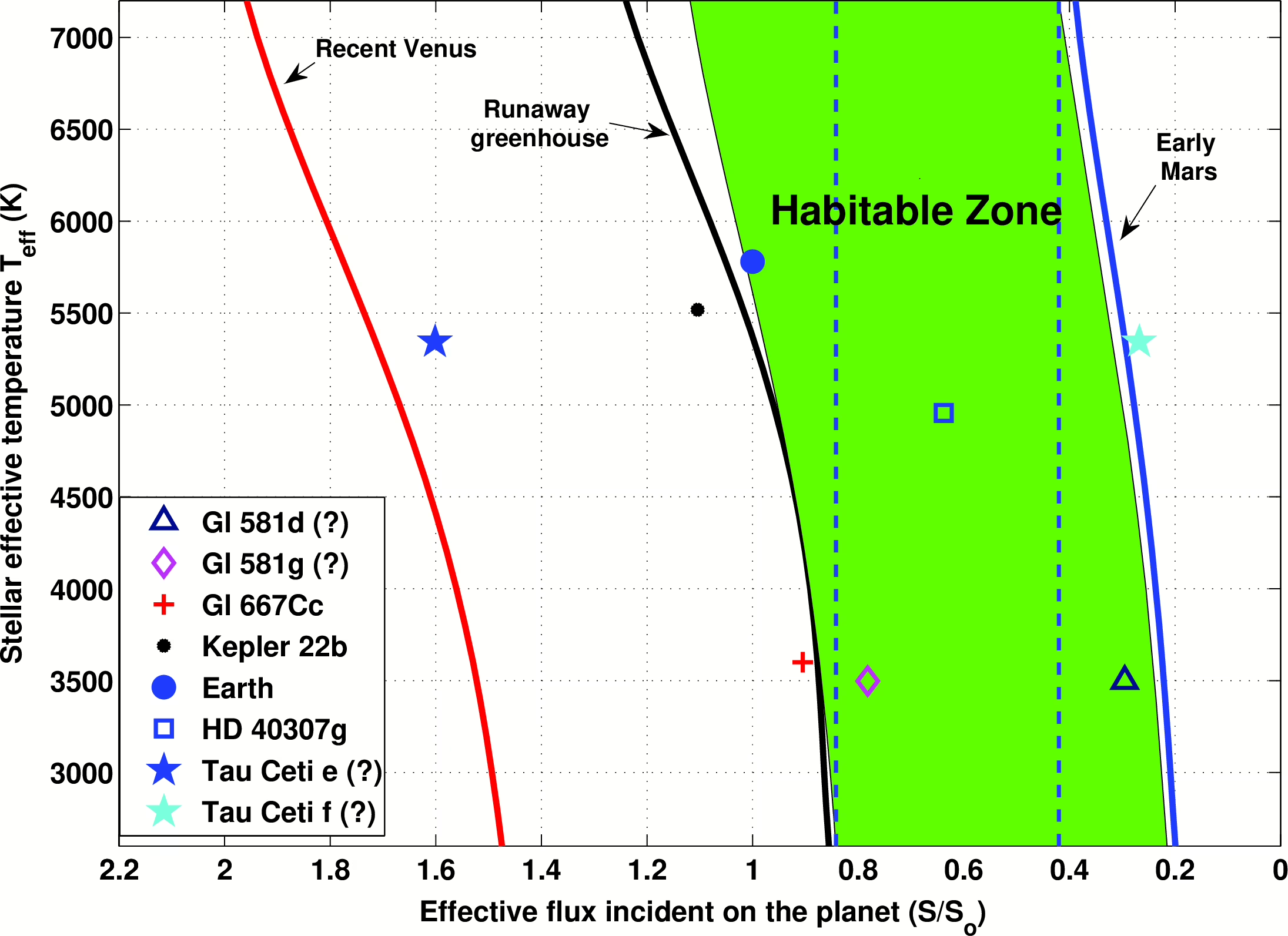
../_images/kopparapu_hz.avif — Fig. 13.47 The **classical habitable zone** as a function of stellar effective temperature and effective stellar flux, from Kopparapu *et al.* [2013]. The green-shaded region is the habitable zone bounded on the inside by the moist greenhouse limit and on the outside by the maximum $\mathrm{CO_2}$ greenhouse limit. Symbols mark known potentially habitable exoplanets including GJ 581 d/g, GJ 667C c, Kepler-22 b, Tau Ceti e/f, and the solar system planets Earth, Venus, and Mars. The “Recent Venus” and “Early Mars” empirical limits are shown by the dotted boundaries.#

Kopparapu et al. [2013] updated these 1D boundaries across stellar effective temperatures, including M dwarfs (Fig. 13.47). Two important caveats apply to these classical estimates.

First, evolutionary history matters rather than snapshot conditions alone. A planet in the habitable zone today may have suffered early runaway greenhouse desiccation (Lecture 9). M dwarf planets spend hundreds of Myr in runaway greenhouse conditions during the pre-main-sequence phase, potentially losing their water inventory [Luger and Barnes, 2015]. Habitability is therefore a trajectory through climate space rather than a static present-day line.

Second, one-dimensional calculations neglect three-dimensional circulation and cloud feedbacks. General circulation models show that cloud feedbacks shift boundaries by 5 to 20% depending on rotation rate, atmospheric composition, and surface albedo [Turbet et al., 2021, Way et al., 2016]. For tidally locked M dwarf planets, substellar clouds extend the inner edge to fluxes well above the 1D moist greenhouse limit. The classical habitable zone is thus a first-order screening tool rather than a precise boundary.

13.5.5. Biosignature gases and the challenge of false positives#

Atmospheric biosignatures are classically identified through disequilibrium gas combinations, mixtures of reactive gases that cannot persist without continuous biological replenishment. On modern Earth, the coexistence of $\mathrm{O_2}$ ($\sim 21\%$) and $\mathrm{CH_4}$ ($\sim 1.8$ ppm) is the canonical example, because both react photochemically within decades and require continuous biological production. Classical biosignature gases include $\mathrm{O_2}$, $\mathrm{O_3}$, $\mathrm{CH_4}$, and $\mathrm{N_2O}$, though a single gas in isolation almost never constitutes a biosignature. Fig. 13.48 shows where these gases absorb: each has bands in the infrared that a transmission or emission spectrum can pick up, which is what makes them observable at all.

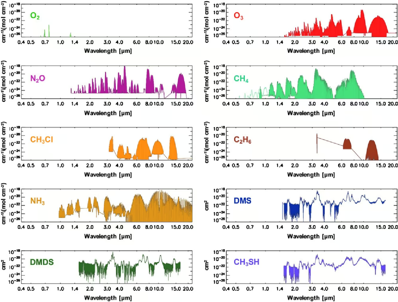
../_images/schwieterman2018_biosignature_gases.avif — Fig. 13.48 Absorption cross-sections from optical to mid-infrared wavelengths (0.4 to 20 $\mu$m) for ten candidate biosignature gases: $\mathrm{O_2}$, $\mathrm{O_3}$, $\mathrm{N_2O}$, $\mathrm{CH_4}$, $\mathrm{CH_3Cl}$, $\mathrm{C_2H_6}$, $\mathrm{NH_3}$, dimethyl sulfide, dimethyl disulfide and $\mathrm{CH_3SH}$. Oxygen absorbs only in narrow optical bands; the others have their strongest features in the infrared. Reproduced from Schwieterman *et al.* [2018].#

The central challenge in biosignature detection is false positives, abiotic processes that mimic biological gas signatures. Wordsworth and Pierrehumbert [2014] showed that water vapour photolysis followed by hydrogen escape can build up substantial abiotic $\mathrm{O_2}$ on dry planets around M dwarfs. Likewise, $\mathrm{CO_2}$ photolysis in dry atmospheres produces abiotic $\mathrm{O_2}$ by splitting $\mathrm{CO_2}$ into CO and O, driven by stellar XUV irradiation. Abiotic $\mathrm{CH_4}$ can similarly arise from volcanic outgassing, hydrothermal serpentinisation reactions, and impact shocks (Lecture 10).

Biosignature identification is fundamentally an inverse problem where candidate gases must be distinguished from abiotic false positives (Lecture 14).

13.5.6. Comparative payoff: the solar system in the exoplanet landscape#

Whether the solar system is typical has been an open question since Lecture 1. If “typical” means the most common configuration in the bias-corrected exoplanet archive, the answer is no. The most common stars are M dwarfs rather than G dwarfs like the Sun. The most common planet class is the sub-Neptune ($2$ to $4\,\Rearth$); the solar system has no planet between Earth ($1\,\Rearth$) and Neptune ($3.88\,\Rearth$). Inner exoplanet systems often form compact peas-in-a-pod configurations ($\sim 5$ to $8$ similarly sized planets within $\sim 0.2$ AU), whereas the solar system has four irregularly spaced terrestrial planets out to $1.5$ AU. The solar system also lacks hot Jupiters or hot Neptunes, and its giant planets occupy wide ($\geq 5$ AU), nearly circular orbits rather than eccentric paths. Comparing Kepler multi-planet architectures directly with the inner solar system highlights this contrast in planet size and orbital spacing (Fig. 13.49).

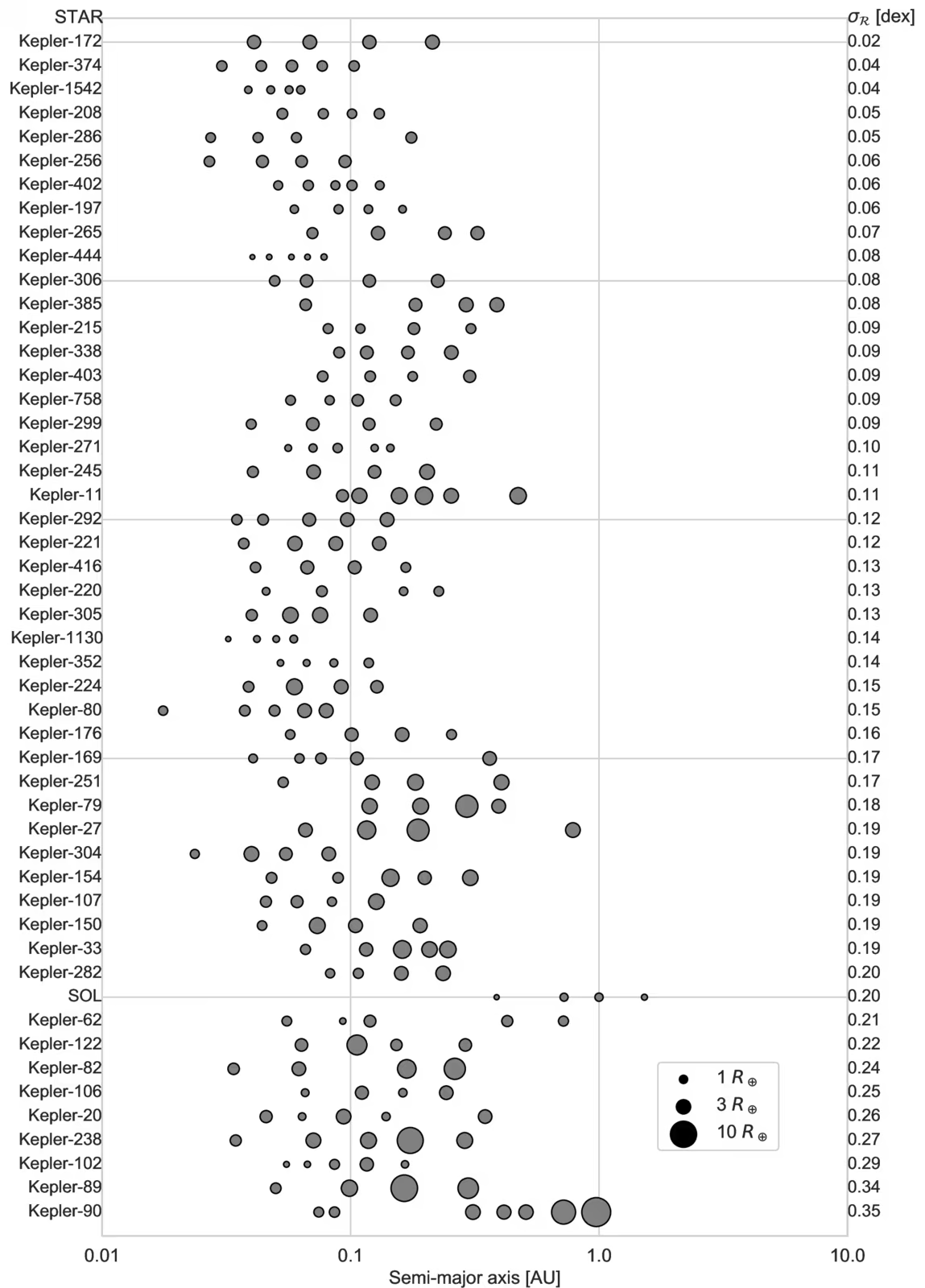
../_images/weiss2023_peas_in_a_pod.avif — Fig. 13.49 Compact multi-planet systems containing four or more transiting planets out to about 1.5 AU, ordered by the dispersion of planet sizes within each system. The solar system terrestrial planets show significantly greater size diversity and wider spacing than typical compact exoplanet architectures. Reproduced from Weiss *et al.* [2023].#

However, the observed archive is shaped by detection biases that work against finding solar system analogues. A Jupiter analogue at $5$ AU produces a radial velocity signal of $\sim 12$ m/s with a 12-year period, requiring more than a decade to detect (fewer than a hundred are known). Saturn analogues at $9.5$ AU and Earth analogues at 1 AU around Sun-like stars sit at the edge of current sensitivity. Whether the solar system is truly rare or merely undersampled in parameter space remains an open question (Lecture 14).

13.5.7. Frontier missions, part 1: surveys and atmospheres (2026–2035)#

PLATO (PLAnetary Transits and Oscillations of stars) is an ESA mission scheduled for launch in January 2027 [Rauer et al., 2014]. Using 26 cameras as a multi-aperture photometric array, PLATO will monitor bright Sun-like stars over 2 to 3 year baselines to detect Earth analogues in the habitable zones of G dwarfs. Ariel will survey approximately 1000 exoplanet atmospheres to provide a statistical census of composition. The Nancy Grace Roman Space Telescope Galactic bulge microlensing survey will deliver $\sim 1400$ bound exoplanets at separations of $\sim 0.5$ to $10$ AU down to lunar masses [Penny et al., 2019].

13.5.8. Frontier missions, part 2: direct imaging of Earth analogues (2030s–2040s)#

The Habitable Worlds Observatory (HWO) is a planned $\sim 6$ m NASA flagship space telescope targeted for launch in the 2040s to directly image Earth analogues. Using a coronagraph or external starshade to achieve contrasts of $10^{-10}$ at sub-arcsecond separations from nearby Sun-like stars, HWO will directly image and obtain spectra of approximately $25$ Earth analogues to search for atmospheric biosignatures. The Large Interferometer For Exoplanets (LIFE) will complement reflected-light imaging by using a mid-infrared nulling interferometer to detect thermal emission from terrestrial exoplanets.

Ground-based Extremely Large Telescopes will further resolve habitable-zone planets around nearby M dwarfs, complementing the space-based direct-imaging concepts of Lecture 14.

13.5.9. Open questions for the next lecture#

A central open question is what constitutes a convincing detection of life on another world. It is debated whether a single biosignature gas, gas abundance ratios, seasonal cycles, or photosynthetic surface features are sufficient. The answer depends on how much we trust atmospheric models and catalogues of false positives. Lecture 14 addresses how to move from a candidate biosignature to detecting life through Bayesian frameworks that combine observational data with planetary context.

13.6. Summary#

Exoplanet science went from the first confirmed detection in 1992 to more than 6000 confirmed planets by 2026, a complete observational revolution in three decades.
Each detection method has a distinct bias: radial velocity and transits favour short periods and large planets, direct imaging targets wide young giants, astrometry finds Jupiter analogues, and microlensing probes wide separations.
The combined transit-plus-radial-velocity measurement breaks the $m \sin i$ degeneracy and gives bulk densities, the central observational quantity that turns exoplanet detections into physical objects with measurable composition.
Kepler showed that planets are common. Most main-sequence stars host at least one planet, and the small-planet population dominates by number. Hot Jupiters occur around only $\sim 1\%$ of Sun-like stars.
The radius valley at $\sim 1.8\,\Rearth$ indicates atmospheric stripping (photoevaporation and core-powered mass loss) that converts sub-Neptunes into bare super-Earth cores.
The hot Neptune desert, the peas-in-a-pod correlation, and the TRAPPIST-1 resonant chain are the other three central architectural results that any planet formation theory must explain.
JWST has made atmospheric characterisation routine, detecting photochemical $\mathrm{SO_2}$ on WASP-39 b, ruling out a thick atmosphere on TRAPPIST-1 b, and testing biosignature claims on K2-18 b.
The solar system is not obviously typical, lacking sub-Neptunes and compact inner systems, though whether it is rare or undersampled remains an open question.
Habitability is a history-dependent trajectory, not a snapshot line on the HR diagram, and biosignature detection is an inverse problem with unavoidable false-positive challenges.
Upcoming missions will push from demography to characterisation of habitable worlds, framing the biosignature detection criteria examined in Lecture 14.

13.7. References#

[Albrecht2022] (1,2,3)

Albrecht, Simon H., Dawson, Rebekah I., and Winn, Joshua N. 2022. “Stellar obliquities in exoplanetary systems.” Publications of the Astronomical Society of the Pacific, 134(1038):082001. doi:10.1088/1538-3873/ac6c09, arXiv:2203.05460, https://ui.adsabs.harvard.edu/abs/2022PASP..134h2001A/abstract.

[Alderson2023] (1,2,3)

Alderson, Lili, Wakeford, Hannah R., Alam, Munazza K., Batalha, Natasha E., Lothringer, Joshua D., Adams Redai, Jea, Barat, Saugata, Brande, Jonathan, Damiano, Mario, Daylan, Tansu, Espinoza, Néstor, Flagg, Laura, Goyal, Jayesh M., Grant, David, Hu, Renyu, Inglis, Julie, Lee, Eliza M.-R., Mikal-Evans, Thomas, Ramos-Rosado, Lakeisha, Roy, Pierre-Alexis, and others. 2023. “Early Release Science of the exoplanet WASP-39b with JWST NIRSpec G395H.” Nature, 614(7949):664–669. doi:10.1038/s41586-022-05591-3, arXiv:2211.10488, https://ui.adsabs.harvard.edu/abs/2023Natur.614..664A/abstract.

[Bell2024]

Bell, Taylor J., Welbanks, Luis, Schlawin, Everett, Line, Michael R., Fortney, Jonathan J., Greene, Thomas P., Ohno, Kazumasa, Parmentier, Vivien, Rauscher, Emily, Beatty, Thomas G., and others. 2024. “Nightside clouds and disequilibrium chemistry on the hot Jupiter WASP-43b.” Nature Astronomy, 8:879–898. doi:10.1038/s41550-024-02230-x, arXiv:2401.13027, https://ui.adsabs.harvard.edu/abs/2024NatAs...8..879B/abstract.

[Borucki2010]

Borucki, William J., Koch, David, Basri, Gibor, Batalha, Natalie, Brown, Timothy, Caldwell, Douglas, and others. 2010. “Kepler planet-detection mission: introduction and first results.” Science, 327(5968):977–980. doi:10.1126/science.1185402, https://ui.adsabs.harvard.edu/abs/2010Sci...327..977B/abstract.

[Bryson2021] (1,2)

Bryson, Steve, Kunimoto, Michelle, Kopparapu, Ravi K., Coughlin, Jeffrey L., Borucki, William J., Koch, David, Silva Aguirre, Víctor, Allen, Christopher, Barentsen, Geert, Batalha, Natalie M., and others. 2021. “The occurrence of rocky habitable-zone planets around solar-like stars from kepler data.” The Astronomical Journal, 161(1):36. doi:10.3847/1538-3881/abc418, arXiv:2010.14812, https://ui.adsabs.harvard.edu/abs/2021AJ....161...36B/abstract.

[Charbonneau2000]

Charbonneau, David, Brown, Timothy M., Latham, David W., and Mayor, Michel. 2000. “Detection of planetary transits across a sun-like star.” The Astrophysical Journal Letters, 529(1):L45–L48. doi:10.1086/312457, arXiv:astro-ph/9911436, https://ui.adsabs.harvard.edu/abs/2000ApJ...529L..45C/abstract.

[ChenKipping2017]

Chen, Jingjing and Kipping, David. 2017. “Probabilistic forecasting of the masses and radii of other worlds.” The Astrophysical Journal, 834(1):17. doi:10.3847/1538-4357/834/1/17, arXiv:1603.08614, https://ui.adsabs.harvard.edu/abs/2017ApJ...834...17C/abstract.

[Doyle2011]

Doyle, Laurance R., Carter, Joshua A., Fabrycky, Daniel C., Slawson, Robert W., Howell, Steve B., Winn, Joshua N., Orosz, Jerome A., Prša, Andrej, Welsh, William F., Quinn, Samuel N., and others. 2011. “Kepler-16: a transiting circumbinary planet.” Science, 333(6049):1602–1606. doi:10.1126/science.1210923, arXiv:1109.3432, https://ui.adsabs.harvard.edu/abs/2011Sci...333.1602D/abstract.

[Dressing2015] (1,2)

Dressing, Courtney D. and Charbonneau, David. 2015. “The occurrence of potentially habitable planets orbiting M dwarfs estimated from the full Kepler dataset and an empirical measurement of the detection sensitivity.” The Astrophysical Journal, 807(1):45. doi:10.1088/0004-637X/807/1/45, arXiv:1501.01623, https://ui.adsabs.harvard.edu/abs/2015ApJ...807...45D/abstract.

[Forget2013]

Forget, F., Wordsworth, R., Millour, E., Madeleine, J.-B., Kerber, L., Leconte, J., Marcq, E., and Haberle, R. M. 2013. “3D modelling of the early martian climate under a denser CO$_2$ atmosphere: temperatures and CO$_2$ ice clouds.” Icarus, 222(1):81–99. doi:10.1016/j.icarus.2012.10.019, arXiv:1210.4216, https://ui.adsabs.harvard.edu/doi/10.1016/j.icarus.2012.10.019/abstract.

[Forget1997]

Forget, François and Pierrehumbert, Raymond T. 1997. “Warming early Mars with carbon dioxide clouds that scatter infrared radiation.” Science, 278(5341):1273–1276. doi:10.1126/science.278.5341.1273, https://ui.adsabs.harvard.edu/abs/1997Sci...278.1273F/abstract.

[Fressin2013]

Fressin, François, Torres, Guillermo, Charbonneau, David, Bryson, Stephen T., Christiansen, Jessie, Dressing, Courtney D., Jenkins, Jon M., Walkowicz, Lucianne M., and Batalha, Natalie M. 2013. “The false positive rate of Kepler and the occurrence of planets.” The Astrophysical Journal, 766(2):81. doi:10.1088/0004-637X/766/2/81, arXiv:1301.0842, https://ui.adsabs.harvard.edu/abs/2013ApJ...766...81F/abstract.

[Fulton2017] (1,2,3)

Fulton, Benjamin J., Petigura, Erik A., Howard, Andrew W., Isaacson, Howard, Marcy, Geoffrey W., Cargile, Phillip A., Hebb, Leslie, Weiss, Lauren M., Johnson, John Asher, Morton, Timothy D., and others. 2017. “The California-Kepler Survey. III. a gap in the radius distribution of small planets.” The Astronomical Journal, 154(3):109. doi:10.3847/1538-3881/aa80eb, arXiv:1703.10375, https://ui.adsabs.harvard.edu/abs/2017AJ....154..109F/abstract.

[Gillon2017] (1,2,3,4)

Gillon, Michaël, Triaud, Amaury H. M. J., Demory, Brice-Olivier, Jehin, Emmanuël, Agol, Eric, Deck, Katherine M., Lederer, Susan M., de Wit, Julien, Burdanov, Artem, Ingalls, James G., and others. 2017. “Seven temperate terrestrial planets around the nearby ultracool dwarf star TRAPPIST-1.” Nature, 542(7642):456–460. doi:10.1038/nature21360, arXiv:1703.01424, https://ui.adsabs.harvard.edu/abs/2017Natur.542..456G/abstract.

[Ginzburg2018] (1,2)

Ginzburg, Sivan, Schlichting, Hilke E., and Sari, Re'em. 2018. “Core-powered mass-loss and the radius distribution of small exoplanets.” Monthly Notices of the Royal Astronomical Society, 476(1):759–765. doi:10.1093/mnras/sty290, arXiv:1708.01621, https://ui.adsabs.harvard.edu/abs/2018MNRAS.476..759G/abstract.

[Glein2024]

Glein, Christopher R. 2024. “Geochemical constraints on the presence of liquid water at depth on hycean candidate K2-18b.” The Astrophysical Journal Letters, 964(1):L19. doi:10.3847/2041-8213/ad3079, arXiv:2403.07761, https://ui.adsabs.harvard.edu/abs/2024ApJ...964L..19G/abstract.

[Greene2023] (1,2,3)

Greene, Thomas P., Bell, Taylor J., Ducrot, Elsa, Dyrek, Achrène, Lagage, Pierre-Olivier, and Fortney, Jonathan J. 2023. “Thermal emission from the Earth-sized exoplanet TRAPPIST-1 b using JWST.” Nature, 618(7963):39–42. doi:10.1038/s41586-023-05951-7, arXiv:2303.14849, https://ui.adsabs.harvard.edu/abs/2023Natur.618...39G/abstract.

[Haffert2019] (1,2,3,4)

Haffert, S. Y., Bohn, A. J., de Boer, J., Snellen, I. A. G., Brinchmann, J., Girard, J. H., Keller, C. U., and Bacon, R. 2019. “Two accreting protoplanets around the young star PDS 70.” Nature Astronomy, 3(8):749–754. doi:10.1038/s41550-019-0780-5, arXiv:1906.01486, https://ui.adsabs.harvard.edu/abs/2019NatAs...3..749H/abstract.

[Henry2000]

Henry, Gregory W., Marcy, Geoffrey W., Butler, R. Paul, and Vogt, Steven S. 2000. “A transiting "51 Peg-like" planet.” The Astrophysical Journal Letters, 529(1):L41–L44. doi:10.1086/312458, arXiv:astro-ph/9912184, https://ui.adsabs.harvard.edu/abs/2000ApJ...529L..41H/abstract.

[Holman2005]

Holman, Matthew J. and Murray, Norman W. 2005. “The use of transit timing to detect terrestrial-mass extrasolar planets.” Science, 307(5713):1288–1291. doi:10.1126/science.1107822, arXiv:astro-ph/0412028, https://ui.adsabs.harvard.edu/abs/2005Sci...307.1288H/abstract.

[Hu2024] (1,2)

Hu, Renyu, Bello-Arufe, Aaron, Zhang, Michael, Paragas, Kimberly, Zilinskas, Mantas, van Buchem, Christiaan, Bess, Michael, Patel, Jayshil, Ito, Yuichi, Damiano, Mario, Scheucher, Markus, Mansfield, Megan, Coulombe, Louis-Philippe, and others. 2024. “A secondary atmosphere on the rocky exoplanet 55 Cancri e.” Nature, 630(8017):609–612. doi:10.1038/s41586-024-07432-x, arXiv:2405.04744, https://ui.adsabs.harvard.edu/abs/2024Natur.630..609H/abstract.

[Kasting1993] (1,2)

Kasting, James F., Whitmire, Daniel P., and Reynolds, Ray T. 1993. “Habitable zones around main sequence stars.” Icarus, 101(1):108–128. doi:10.1006/icar.1993.1010, https://ui.adsabs.harvard.edu/abs/1993Icar..101..108K/abstract.

[Keppler2018]

Keppler, M., Benisty, M., Müller, A., Henning, Th., van Boekel, R., Cantalloube, F., Ginski, C., van Holstein, R. G., Maire, A.-L., Pohl, A., Samland, M., Avenhaus, H., Baudino, J.-L., Boccaletti, A., de Boer, J., Brandner, W., Cardenas, M. C., Carson, J., Casassus, S., Chauvin, G., and others. 2018. “Discovery of a planetary-mass companion within the gap of the transition disk around PDS 70.” Astronomy & Astrophysics, 617:A44. doi:10.1051/0004-6361/201832957, arXiv:1806.11568, https://ui.adsabs.harvard.edu/abs/2018A%26A...617A..44K/abstract.

[Kitzmann2016]

Kitzmann, D. 2016. “Revisiting the scattering greenhouse effect of CO$_2$ ice clouds.” The Astrophysical Journal Letters, 817(2):L18. doi:10.3847/2041-8205/817/2/L18, arXiv:1601.01209, https://ui.adsabs.harvard.edu/doi/10.3847/2041-8205/817/2/L18/abstract.

[Kitzmann2017]

Kitzmann, D. 2017. “Clouds in the atmospheres of extrasolar planets. V. The impact of CO$_2$ ice clouds on the outer boundary of the habitable zone.” Astronomy & Astrophysics, 600:A111. doi:10.1051/0004-6361/201630029, arXiv:1701.07513, https://ui.adsabs.harvard.edu/doi/10.1051/0004-6361/201630029/abstract.

[Kopparapu2013] (1,2,3,4)

Kopparapu, Ravi Kumar, Ramirez, Ramses, Kasting, James F., Eymet, Vincent, Robinson, Tyler D., Mahadevan, Suvrath, Terrien, Ryan C., Domagal-Goldman, Shawn, Meadows, Victoria, and Deshpande, Rohit. 2013. “Habitable zones around main-sequence stars: new estimates.” The Astrophysical Journal, 765(2):131. doi:10.1088/0004-637X/765/2/131, arXiv:1301.6674, https://ui.adsabs.harvard.edu/abs/2013ApJ...765..131K/abstract.

[Kreidberg2014]

Kreidberg, Laura, Bean, Jacob L., Désert, Jean-Michel, Benneke, Björn, Deming, Drake, Stevenson, Kevin B., Seager, Sara, Berta-Thompson, Zachory, Seifahrt, Andreas, and Homeier, Derek. 2014. “Clouds in the atmosphere of the super-Earth exoplanet GJ 1214b.” Nature, 505(7481):69–72. doi:10.1038/nature12888, arXiv:1401.0022, https://ui.adsabs.harvard.edu/abs/2014Natur.505...69K/abstract.

[Lagrange2010] (1,2)

Lagrange, A.-M., Bonnefoy, M., Chauvin, G., Apai, D., Ehrenreich, D., Boccaletti, A., Gratadour, D., Rouan, D., Mouillet, D., Lacour, S., and Kasper, M. 2010. “A giant planet imaged in the disk of the young star β Pictoris.” Science, 329(5987):57–59. doi:10.1126/science.1187187, arXiv:1006.3314, https://ui.adsabs.harvard.edu/abs/2010Sci...329...57L/abstract.

[Lichtenberg2025]

Lichtenberg, Tim, Shorttle, Oliver, Teske, Johanna, and Kempton, Eliza M.-R. 2025. “Constraining exoplanet interiors using observations of their atmospheres.” Science, 390:eads3360. doi:10.1126/science.ads3360, https://ui.adsabs.harvard.edu/abs/2025Sci...390S3660L/abstract.

[LugerBarnes2015] (1,2)

Luger, R. and Barnes, R. 2015. “Extreme water loss and abiotic O₂ buildup on planets throughout the habitable zones of M dwarfs.” Astrobiology, 15(2):119–143. doi:10.1089/ast.2014.1231, arXiv:1411.7412, https://ui.adsabs.harvard.edu/abs/2015AsBio..15..119L/abstract.

[Luger2017]

Luger, Rodrigo, Sestovic, Marko, Kruse, Ethan, Grimm, Simon L., Demory, Brice-Olivier, Agol, Eric, Bolmont, Emeline, Fabrycky, Daniel, Fernandes, Catarina S., Van Grootel, Valérie, and others. 2017. “A seven-planet resonant chain in TRAPPIST-1.” Nature Astronomy, 1:0129. doi:10.1038/s41550-017-0129, https://ui.adsabs.harvard.edu/abs/2017NatAs...1E.129L/abstract.

[LustigYaeger2023] (1,2)

Lustig-Yaeger, Jacob, Fu, Guangwei, May, Erin M., Ceballos, Kristin N. O., Moran, Sarah E., Peacock, Sarah, Stevenson, Kevin B., Kirk, James, López-Morales, Mercedes, MacDonald, Ryan J., Mayorga, L. C., Sing, David K., Sotzen, Kristin S., Valenti, Jeff A., Adams Redai, Jea I., Alam, Munazza K., Batalha, Natasha E., Bennett, Katherine A., Gonzalez-Quiles, Junellie, Lewis, Nikole K., and others. 2023. “A JWST transmission spectrum of the nearby Earth-sized exoplanet LHS 475 b.” Nature Astronomy, 7:1317–1328. doi:10.1038/s41550-023-02064-z, arXiv:2301.04191, https://ui.adsabs.harvard.edu/abs/2023NatAs...7.1317L/abstract.

[Madhusudhan2021]

Madhusudhan, Nikku, Piette, Anjali A. A., and Constantinou, Savvas. 2021. “Habitability and biosignatures of Hycean worlds.” The Astrophysical Journal, 918(1):1. doi:10.3847/1538-4357/abfd9c, arXiv:2108.10888, https://ui.adsabs.harvard.edu/abs/2021ApJ...918....1M/abstract.

[Madhusudhan2023] (1,2)

Madhusudhan, Nikku, Sarkar, Subhajit, Constantinou, Savvas, Holmberg, Måns, Piette, Anjali A. A., and Moses, Julianne I. 2023. “Carbon-bearing molecules in a possible Hycean atmosphere.” The Astrophysical Journal Letters, 956(1):L13. doi:10.3847/2041-8213/acf577, arXiv:2309.05566, https://ui.adsabs.harvard.edu/abs/2023ApJ...956L..13M/abstract.

[Marois2008] (1,2)

Marois, Christian, Macintosh, Bruce, Barman, Travis, Zuckerman, B., Song, Inseok, Patience, Jennifer, Lafrenière, David, and Doyon, René. 2008. “Direct imaging of multiple planets orbiting the star HR 8799.” Science, 322(5906):1348–1352. doi:10.1126/science.1166585, arXiv:0811.2606, https://ui.adsabs.harvard.edu/abs/2008Sci...322.1348M/abstract.

[Mayor2003]

Mayor, Michel, Pepe, Francesco, Queloz, Didier, Bouchy, François, Rupprecht, Gero, Lo Curto, Gaspare, Avila, Gerardo, Benz, Willy, Bertaux, Jean-Loup, Bonfils, Xavier, and others. 2003. “Setting new standards with HARPS.” The Messenger, 114:20–24. https://ui.adsabs.harvard.edu/abs/2003Msngr.114...20M/abstract.

[MayorQueloz1995]

Mayor, Michel and Queloz, Didier. 1995. “A Jupiter-mass companion to a solar-type star.” Nature, 378:355–359. doi:10.1038/378355a0, https://ui.adsabs.harvard.edu/abs/1995Natur.378..355M/abstract.

[Mazeh2016] (1,2)

Mazeh, Tsevi, Holczer, Tomer, and Faigler, Shay. 2016. “Dearth of short-period Neptunian exoplanets: a desert in period-mass and period-radius planes.” Astronomy & Astrophysics, 589:A75. doi:10.1051/0004-6361/201528065, arXiv:1602.07843, https://ui.adsabs.harvard.edu/abs/2016A%26A...589A..75M/abstract.

[Moran2023]

Moran, Sarah E., Stevenson, Kevin B., Sing, David K., MacDonald, Ryan J., Kirk, James, Lustig-Yaeger, Jacob, Peacock, Sarah, Mayorga, L. C., Bennett, Katherine A., López-Morales, Mercedes, and others. 2023. “High tide or riptide on the cosmic shoreline? A water-rich atmosphere or stellar contamination for the warm super-Earth GJ 486b from JWST observations.” The Astrophysical Journal Letters, 948(1):L11. doi:10.3847/2041-8213/accb9c, arXiv:2305.00868, https://ui.adsabs.harvard.edu/abs/2023ApJ...948L..11M/abstract.

[OwenWu2013] (1,2,3)

Owen, James E. and Wu, Yanqin. 2013. “Kepler planets: a tale of evaporation.” The Astrophysical Journal, 775(2):105. doi:10.1088/0004-637X/775/2/105, arXiv:1206.2367, https://ui.adsabs.harvard.edu/abs/2013ApJ...775..105O/abstract.

[Penny2019] (1,2)

Penny, Matthew T., Gaudi, B. Scott, Kerins, Eamonn, Rattenbury, Nicholas J., Mao, Shude, Robin, Annie C., and Calchi Novati, Sebastiano. 2019. “Predictions of the WFIRST microlensing survey. I. bound planet detection rates.” The Astrophysical Journal Supplement Series, 241(1):3. doi:10.3847/1538-4365/aafb69, arXiv:1808.02490, https://ui.adsabs.harvard.edu/abs/2019ApJS..241....3P/abstract.

[Pepe2021]

Pepe, Francesco, Cristiani, Stefano, Rebolo, Rafael, Santos, Nuno C., Dekker, Hans, Cabral, Alexandre, Di Marcantonio, Paolo, Figueira, Pedro, Lo Curto, Gaspare, Lovis, Christophe, and others. 2021. “ESPRESSO at VLT. on-sky performance and first results.” Astronomy & Astrophysics, 645:A96. doi:10.1051/0004-6361/202038306, arXiv:2010.00316, https://ui.adsabs.harvard.edu/abs/2021A%26A...645A..96P/abstract.

[Perryman2014]

Perryman, Michael, Hartman, Joel, Bakos, Gáspár Á., and Lindegren, Lennart. 2014. “Astrometric exoplanet detection with Gaia.” The Astrophysical Journal, 797(1):14. doi:10.1088/0004-637X/797/1/14, arXiv:1411.1173, https://ui.adsabs.harvard.edu/abs/2014ApJ...797...14P/abstract.

[Petigura2018] (1,2)

Petigura, Erik A., Marcy, Geoffrey W., Winn, Joshua N., Weiss, Lauren M., Fulton, Benjamin J., Howard, Andrew W., Sinukoff, Evan, Isaacson, Howard, Morton, Timothy D., and Johnson, John Asher. 2018. “The California-Kepler Survey. IV. metal-rich stars host a greater diversity of planets.” The Astronomical Journal, 155(2):89. doi:10.3847/1538-3881/aaa54c, arXiv:1712.04042, https://ui.adsabs.harvard.edu/abs/2018AJ....155...89P/abstract.

[Pidhorodetska2026]

Pidhorodetska, Daria, Schwieterman, Edward W., Fauchez, Thomas J., and Turbet, Martin. 2026. “High-CO$_2$ climates and observables in the outer habitable zone.” The Astrophysical Journal, 1009(2):179. doi:10.3847/1538-4357/ae9869, arXiv:2609.36697, https://ui.adsabs.harvard.edu/doi/10.3847/1538-4357/ae9869/abstract.

[Pollack1996]

Pollack, James B., Hubickyj, Olenka, Bodenheimer, Peter, Lissauer, Jack J., Podolak, Morris, and Greenzweig, Yuval. 1996. “Formation of the giant planets by concurrent accretion of solids and gas.” Icarus, 124(1):62–85. doi:10.1006/icar.1996.0190, https://ui.adsabs.harvard.edu/abs/1996Icar..124...62P/abstract.

[Rauer2014] (1,2)

Rauer, Heike, Catala, Claude, Aerts, Conny, Appourchaux, Thierry, Benz, Willy, Brandeker, Alexis, Christensen-Dalsgaard, Jørgen, Deleuil, Magali, Gizon, Laurent, and others. 2014. “The PLATO 2.0 mission.” Experimental Astronomy, 38(1–2):249–330. doi:10.1007/s10686-014-9383-4, arXiv:1310.0696, https://ui.adsabs.harvard.edu/abs/2014ExA....38..249R/abstract.

[Rustamkulov2023] (1,2)

Rustamkulov, Z., Sing, D. K., Mukherjee, S., May, E. M., Kirk, J., Schlawin, E., Line, M. R., Piaulet, C., Carter, A. L., Batalha, N. E., and others. 2023. “Early Release Science of the exoplanet WASP-39b with JWST NIRSpec PRISM.” Nature, 614(7949):659–663. doi:10.1038/s41586-022-05677-y, arXiv:2211.10487, https://ui.adsabs.harvard.edu/abs/2023Natur.614..659R/abstract.

[Schwieterman2018]

Schwieterman, Edward W., Kiang, Nancy Y., Parenteau, Mary N., Harman, Chester E., DasSarma, Shiladitya, Fisher, Theresa M., Arney, Giada N., Hartnett, Hilairy E., Reinhard, Christopher T., Olson, Stephanie L., Meadows, Victoria S., Cockell, Charles S., Walker, Sara I., Grenfell, John Lee, Hegde, Siddharth, Rugheimer, Sarah, Hu, Renyu, and Lyons, Timothy W. 2018. “Exoplanet biosignatures: a review of remotely detectable signs of life.” Astrobiology, 18(6):663–708. doi:10.1089/ast.2017.1729, arXiv:1705.05791, https://ui.adsabs.harvard.edu/abs/2018AsBio..18..663S/abstract.

[Shorttle2024] (1,2)

Shorttle, Oliver, Jordan, Sean, Nicholls, Harrison, Lichtenberg, Tim, and Bower, Dan J. 2024. “Distinguishing oceans of water from magma on mini-Neptune K2-18b.” The Astrophysical Journal Letters, 962(1):L8. doi:10.3847/2041-8213/ad206e, arXiv:2401.05864, https://ui.adsabs.harvard.edu/abs/2024ApJ...962L...8S/abstract.

[Sing2016] (1,2)

Sing, David K., Fortney, Jonathan J., Nikolov, Nikolay, Wakeford, Hannah R., Kataria, Tiffany, Evans, Thomas M., Aigrain, Suzanne, Ballester, Gilda E., Burrows, Adam S., Deming, Drake, Désert, Jean-Michel, Gibson, Neale P., Henry, Gregory W., Huitson, Catherine M., Knutson, Heather A., Lecavelier des Etangs, Alain, Pont, Frederic, Showman, Adam P., Vidal-Madjar, Alfred, Williamson, Michael H., and Wilson, Paul A. 2016. “A continuum from clear to cloudy hot-Jupiter exoplanets without primordial water depletion.” Nature, 529(7584):59–62. doi:10.1038/nature16068, arXiv:1512.04341, https://ui.adsabs.harvard.edu/abs/2016Natur.529...59S/abstract.

[Tsai2023] (1,2)

Tsai, Shang-Min, Lee, Elspeth K. H., Powell, Diana, Gao, Peter, Zhang, Xi, Moses, Julianne, Hébrard, Eric, Venot, Olivia, Parmentier, Vivien, Jordan, Sean, Hu, Renyu, Alam, Munazza K., Alderson, Lili, Batalha, Natalie M., Bean, Jacob L., Benneke, Björn, Bierson, Carver J., Brady, Ryan P., Carone, Ludmila, Carter, Aarynn L., and others. 2023. “Photochemically produced SO₂ in the atmosphere of WASP-39b.” Nature, 617(7961):483–487. doi:10.1038/s41586-023-05902-2, arXiv:2211.10490, https://ui.adsabs.harvard.edu/abs/2023Natur.617..483T/abstract.

[Turbet2021]

Turbet, Martin, Bolmont, Emeline, Chaverot, Guillaume, Ehrenreich, David, Leconte, Jérémy, and Marcq, Emmanuel. 2021. “Day–night cloud asymmetry prevents early oceans on Venus but not on Earth.” Nature, 598(7880):276–280. doi:10.1038/s41586-021-03873-w, https://ui.adsabs.harvard.edu/abs/2021Natur.598..276T/abstract.

[Turbet2017]

Turbet, Martin, Forget, François, Leconte, Jérémy, Charnay, Benjamin, and Tobie, Gabriel. 2017. “CO$_2$ condensation is a serious limit to the deglaciation of Earth-like planets.” Earth and Planetary Science Letters, 476:11–21. doi:10.1016/j.epsl.2017.07.050, arXiv:1703.04624, https://ui.adsabs.harvard.edu/doi/10.1016/j.epsl.2017.07.050/abstract.

[VanEylen2018] (1,2,3)

Van Eylen, V., Agentoft, Camilla, Lundkvist, M. S., Kjeldsen, H., Owen, J. E., Fulton, B. J., Petigura, E., and Snellen, I. 2018. “An asteroseismic view of the radius valley: stripped cores, not born rocky.” Monthly Notices of the Royal Astronomical Society, 479(4):4786–4795. doi:10.1093/mnras/sty1783, arXiv:1710.05398, https://ui.adsabs.harvard.edu/abs/2018MNRAS.479.4786V/abstract.

[Way2016]

Way, Michael J., Del Genio, Anthony D., Kiang, Nancy Y., Sohl, Linda E., Grinspoon, David H., Aleinov, Igor, Kelley, Maxwell, and Clune, Thomas. 2016. “Was Venus the first habitable world of our solar system?.” Geophysical Research Letters, 43(16):8376–8383. doi:10.1002/2016GL069790, https://ui.adsabs.harvard.edu/abs/2016GeoRL..43.8376W/abstract.

[Weiss2018] (1,2,3)

Weiss, Lauren M., Marcy, Geoffrey W., Petigura, Erik A., Fulton, Benjamin J., Howard, Andrew W., Winn, Joshua N., Isaacson, Howard T., Morton, Timothy D., Hirsch, Lea A., Sinukoff, Evan J., Cumming, Andrew, Hebb, Leslie, and Cargile, Phillip A. 2018. “The California-Kepler Survey. V. peas in a pod: planets in a Kepler multi-planet system are similar in size and regularly spaced.” The Astronomical Journal, 155(1):48. doi:10.3847/1538-3881/aa9ff6, arXiv:1706.06204, https://ui.adsabs.harvard.edu/abs/2018AJ....155...48W/abstract.

[Weiss2023]

Weiss, Lauren M., Millholland, Sarah C., Petigura, Erik A., Adams, Fred C., Batygin, Konstantin, Bloch, Anthony M., and Becker, Juliette. 2023. “Architectures of compact multi-planet systems: diversity and uniformity.” In Inutsuka, Shu-ichiro, Aikawa, Yuri, Muto, Takayuki, Tomida, Kengo, and Tamura, Motohide, editors, Protostars and Planets VII. ASP Conference Series. doi:10.48550/arXiv.2203.10076, arXiv:2203.10076, https://ui.adsabs.harvard.edu/abs/2023ASPC..534..863W/abstract.

[Winn2010] (1,2)

Winn, Joshua N. 2010. “Exoplanet transits and occultations.” arXiv e-prints. Chapter in Exoplanets, ed. S. Seager (Univ. Arizona Press). arXiv:1001.2010, https://ui.adsabs.harvard.edu/abs/2010arXiv1001.2010W/abstract.

[Wogan2024]

Wogan, Nicholas F., Batalha, Natasha E., Zahnle, Kevin J., Krissansen-Totton, Joshua, Tsai, Shang-Min, and Hu, Renyu. 2024. “JWST observations of K2-18b can be explained by a gas-rich mini-Neptune with no habitable surface.” The Astrophysical Journal Letters, 963(1):L7. doi:10.3847/2041-8213/ad2616, arXiv:2401.11082, https://ui.adsabs.harvard.edu/abs/2024ApJ...963L...7W/abstract.

[Wolszczan1994]

Wolszczan, Aleksander. 1994. “Confirmation of Earth-mass planets orbiting the millisecond pulsar PSR B1257+12.” Science, 264(5158):538–542. doi:10.1126/science.264.5158.538, https://ui.adsabs.harvard.edu/abs/1994Sci...264..538W/abstract.

[Wolszczan1992] (1,2,3)

Wolszczan, Aleksander and Frail, Dale A. 1992. “A planetary system around the millisecond pulsar PSR1257+12.” Nature, 355:145–147. doi:10.1038/355145a0, https://ui.adsabs.harvard.edu/abs/1992Natur.355..145W/abstract.

[Wordsworth2014]

Wordsworth, R. D. and Pierrehumbert, R. T. 2014. “Abiotic oxygen-dominated atmospheres on terrestrial habitable zone planets.” The Astrophysical Journal Letters, 785(2):L20. doi:10.1088/2041-8205/785/2/L20, arXiv:1403.2713, https://ui.adsabs.harvard.edu/abs/2014ApJ...785L..20W/abstract.

[Yang2013]

Yang, Jun, Cowan, Nicolas B., and Abbot, Dorian S. 2013. “Stabilizing cloud feedback dramatically expands the habitable zone of tidally locked planets.” The Astrophysical Journal Letters, 771(2):L45. doi:10.1088/2041-8205/771/2/L45, arXiv:1307.0515, https://ui.adsabs.harvard.edu/abs/2013ApJ...771L..45Y/abstract.

[Zieba2023]

Zieba, Sebastian, Kreidberg, Laura, Ducrot, Elsa, Gillon, Michaël, Morley, Caroline, Schaefer, Laura, Tamburo, Patrick, Koll, Daniel D. B., Lustig-Yaeger, Jacob, Lyu, Renyu, and others. 2023. “No thick carbon dioxide atmosphere on the rocky exoplanet TRAPPIST-1 c.” Nature, 620(7975):746–749. doi:10.1038/s41586-023-06232-z, arXiv:2306.10150, https://ui.adsabs.harvard.edu/abs/2023Natur.620..746Z/abstract.

[GaiaDR3]

Gaia Collaboration, Arenou, F., Babusiaux, C., Barstow, M. A., Faigler, S., Jorissen, A., Kervella, P., Mazeh, T., Panuzzo, P., Sahlmann, J., and others. 2023. “Gaia Data Release 3. Stellar multiplicity, a teaser for the hidden treasure.” Astronomy & Astrophysics, 674:A34. doi:10.1051/0004-6361/202243782, arXiv:2206.05595, https://ui.adsabs.harvard.edu/abs/2023A%26A...674A..34G/abstract.

[NASAExoplanetArchive2026]

NASA Exoplanet Archive. 2026. NASA Exoplanet Archive: Confirmed Planets Table. NASA Exoplanet Science Institute, Caltech/IPAC. Accessed 2026-04-16. doi:10.26133/NEA1, https://exoplanetarchive.ipac.caltech.edu/.

[NASAExoArchive2025]

NASA Exoplanet Science Institute. 2025. NASA Exoplanet Archive. NASA Exoplanet Science Institute / Caltech-IPAC. Accessed 2026 March; planet counts updated continuously. https://exoplanetarchive.ipac.caltech.edu/.