6. Atmospheres II: Clouds, Weather, & Climate

Learning objectives: By the end of this lecture, you will be able to derive the Clausius-Clapeyron equation and apply it to predict cloud formation conditions, explain atmospheric circulation patterns using the Coriolis effect and geostrophic balance, describe weather phenomena across the solar system, and discuss long-term climate evolution including the faint young Sun paradox and the carbonate-silicate cycle.

See also

Slides: Download Lecture 6 (PDF)

6.1. Cloud formation

In Lecture 5, we studied the vertical structure of atmospheres: how pressure and temperature vary with altitude, and how radiation and convection control the energy balance. We now turn to what happens when the air becomes too cold to hold all of its vapour: clouds form.

6.1.1. Saturation and condensation

Every gas has a maximum amount of vapour that the surrounding air can hold at a given temperature. This maximum is set by the saturation vapour pressure \(P_{\mathrm{sat}}(T)\), the partial pressure at which the rate of evaporation from a liquid (or solid) surface equals the rate of condensation back onto it. When the actual partial pressure of a vapour exceeds \(P_{\mathrm{sat}}\), the air is supersaturated and condensation is thermodynamically favoured [Pierrehumbert, 2010].

The key property of \(P_{\mathrm{sat}}(T)\) is its strong temperature dependence: it increases roughly exponentially with temperature. A parcel of air that is unsaturated at the warm surface can become saturated simply by cooling (for example, by rising and expanding adiabatically). The temperature at which a parcel first reaches saturation is called the dew point (for condensation to liquid) or the frost point (for deposition to ice).

The relative humidity is defined as the ratio of the actual vapour pressure to the saturation vapour pressure:

\[ \mathrm{RH} = \frac{P_{\mathrm{vapour}}}{P_{\mathrm{sat}}(T)} \times 100\% \]

When \(\mathrm{RH} = 100\%\), the air is saturated; when \(\mathrm{RH} > 100\%\), it is supersaturated and condensation can occur. The exponential temperature dependence of \(P_\mathrm{sat}\) for the principal condensable species in solar system atmospheres is shown in Fig. 6.1.

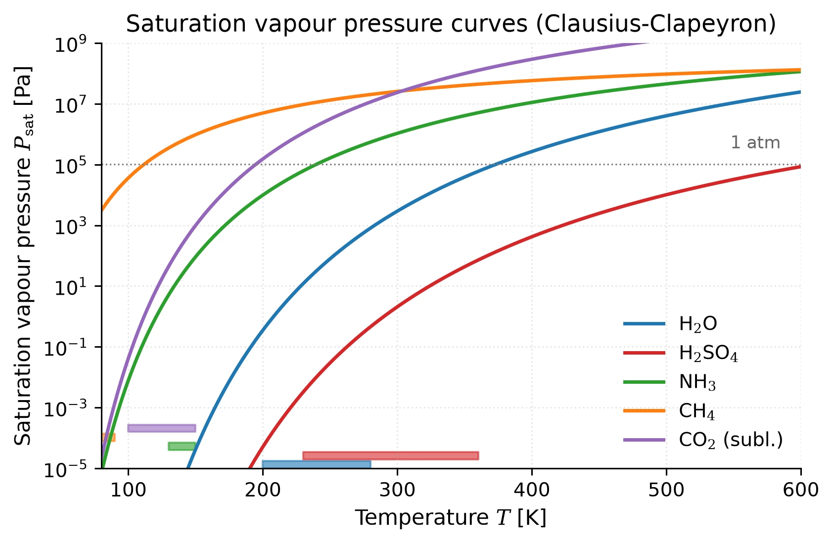
Fig. 6.1 Saturation vapour pressure \(P_{\mathrm{sat}}(T)\) as a function of temperature for the major condensable species in solar system atmospheres: \(\mathrm{H_2O}\), \(\mathrm{H_2SO_4}\), \(\mathrm{NH_3}\), \(\mathrm{CH_4}\), and \(\mathrm{CO_2}\) (sublimation curve). The exponential temperature dependence predicted by the Clausius-Clapeyron equation (Eq. (6.1)) is evident on the logarithmic vertical axis. Coloured bands at the bottom mark the temperature ranges over which each species condenses: \(\mathrm{H_2O}\) on Earth and Mars; \(\mathrm{H_2SO_4}\) on Venus; \(\mathrm{NH_3}\) on Jupiter and Saturn; \(\mathrm{CH_4}\) on Titan, Uranus, and Neptune; and \(\mathrm{CO_2}\) on Mars. Plot generated from thermodynamic data in [Catling and Kasting, 2017] and [Pierrehumbert, 2010]. Course-original figure.

6.1.2. Nucleation

Even when air is supersaturated, condensation does not happen instantly. Forming a new droplet requires overcoming an energy barrier: the surface energy of the tiny embryonic droplet. This process is called nucleation [Catling and Kasting, 2017].

• Homogeneous nucleation (forming droplets from vapour alone, without any pre-existing surface) requires very high supersaturations (RH \(\gg\) 100%) and is extremely rare in planetary atmospheres.

• Heterogeneous nucleation (condensation onto pre-existing particles called condensation nuclei: dust grains, volcanic aerosols, sea salt, soot, cosmic ray ions) occurs at much lower supersaturations (RH \(\gtrsim\) 100%) and is the dominant cloud formation mechanism on all planets.

The availability of condensation nuclei therefore controls where and how easily clouds form. On Earth, the oceans and biosphere provide abundant nuclei. On Mars, wind-lofted mineral dust serves the same role. On the giant planets, photochemical hazes, aerosol particles formed when ultraviolet sunlight breaks apart atmospheric molecules whose fragments recombine into new compounds, provide nuclei for cloud formation deeper down. How solute condensation nuclei lower the supersaturation barrier relative to homogeneous nucleation is shown by the Köhler curves in Fig. 6.2.

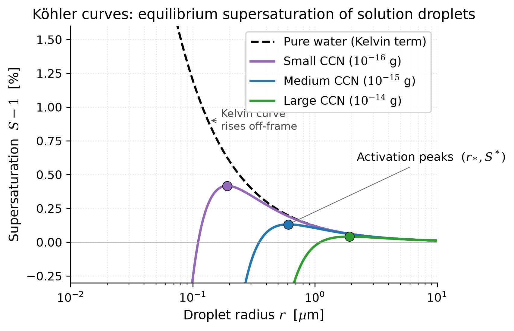
Fig. 6.2 Köhler curves: equilibrium supersaturation \(S - 1\) at which a solution droplet of radius \(r\) neither grows nor evaporates. The dashed black curve is the pure-water Kelvin term, \(S = 1 + A/r\), which formalises the energy cost of homogeneous nucleation: the equilibrium supersaturation, computed from the same term above the top of the plotted range, is already \(S - 1 \approx 12\%\) at \(r = 10^{-2}\,\mu\)m and climbs toward \(\sim\)100% at the nanometre scale of freshly formed embryos, far beyond anything sustained in planetary atmospheres. The coloured curves show the Köhler form \(S = 1 + A/r - B/r^3\) for solution droplets condensed on dry condensation nuclei (CCN) of three solute masses spanning the typical atmospheric range, \(m_s = 10^{-16}\), \(10^{-15}\), and \(10^{-14}\) g [Pruppacher and Klett, 1997]. The Raoult term \(-B/r^3\) pushes the equilibrium curve below the Kelvin curve, so heterogeneous nucleation activates at peak supersaturations of only \(\sim\)0.04-0.4%, easily reached in adiabatically cooled updraughts. This is why heterogeneous nucleation dominates on every planet with abundant aerosols. Adapted from the formulation in [Catling and Kasting, 2017]. Course-original figure.

6.1.3. The lifting condensation level

As an air parcel rises through the troposphere, it cools at the dry adiabatic lapse rate \(\Gamma_d = g/c_p\) (Eq. (5.6) from Lecture 5). Its vapour mixing ratio is conserved during adiabatic ascent, so its vapour pressure falls only in proportion to the total pressure, while \(P_{\mathrm{sat}}(T)\) drops exponentially as the temperature falls. At the altitude where the parcel temperature has cooled enough that \(P_{\mathrm{vapour}} = P_{\mathrm{sat}}(T)\), condensation begins. This altitude is the lifting condensation level (LCL) and marks the cloud base.

Above the LCL, the rising parcel releases latent heat as vapour condenses, warming the parcel relative to the dry adiabat. This gives the moist adiabatic lapse rate, which is shallower than the dry adiabat (\(\sim\)9.8 K km\(^{-1}\)): a representative value in Earth’s warm lower troposphere is \(\sim\)5 K km\(^{-1}\), and the observed tropospheric mean of \(\sim\)6.5 K km\(^{-1}\) lies between the two limits (Lecture 5). The latent heat release also provides buoyancy, driving vigorous convection in moist atmospheres: the mechanism behind thunderstorms, hurricanes, and the towering cumulonimbus clouds on Earth (Fig. 6.3).

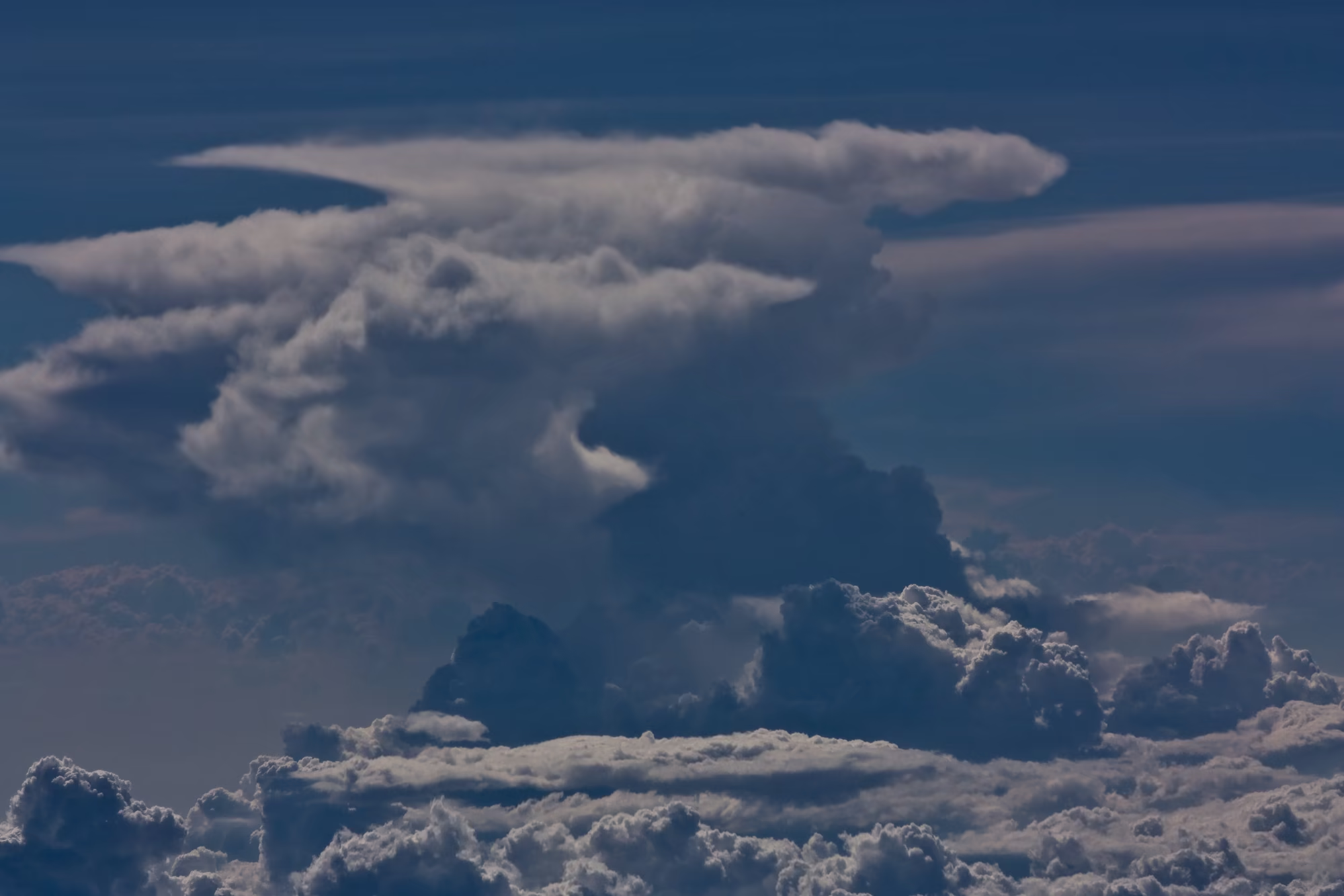
Fig. 6.3 A cumulonimbus cloud spreading into a flat anvil (incus) at its top, seen from above the surrounding cloud deck. Latent heat released by condensing water vapour keeps the rising air warmer than its surroundings and drives the convective tower upward. The tower climbs until it reaches the tropopause, where the stable stratosphere above stops the ascent and the cloud spreads sideways into the anvil. The anvil top therefore marks the altitude where convective buoyancy ends. Credit: Eulenjäger, CC BY-SA 3.0, via Wikimedia Commons.

6.1.4. Cloud types depend on the condensing species

What condenses depends on what vapour is present and at what temperature. This varies dramatically across the solar system:

• Earth: \(\mathrm{H_2O}\) clouds (liquid droplets and ice crystals), with cloud base at \(\sim\)1–2 km

• Venus: \(\mathrm{H_2SO_4}\) (sulfuric acid) droplets at 48–70 km altitude

• Mars: \(\mathrm{CO_2}\) ice and \(\mathrm{H_2O}\) ice clouds at high altitude

• Titan: \(\mathrm{CH_4}\) and \(\mathrm{C_2H_6}\) (ethane) clouds in the lower troposphere (about 8 to 30 km)

• Jupiter/Saturn: Layered \(\mathrm{NH_3}\), \(\mathrm{NH_4SH}\), and \(\mathrm{H_2O}\) clouds at successively deeper levels

The physics of cloud formation is the same in every case: the Clausius-Clapeyron equation governs all of them. The difference is which species condenses and at what temperature.

Fig. 6.4 compares the condensing species and cloud altitudes of the five bodies in separate panels (the height scales differ).

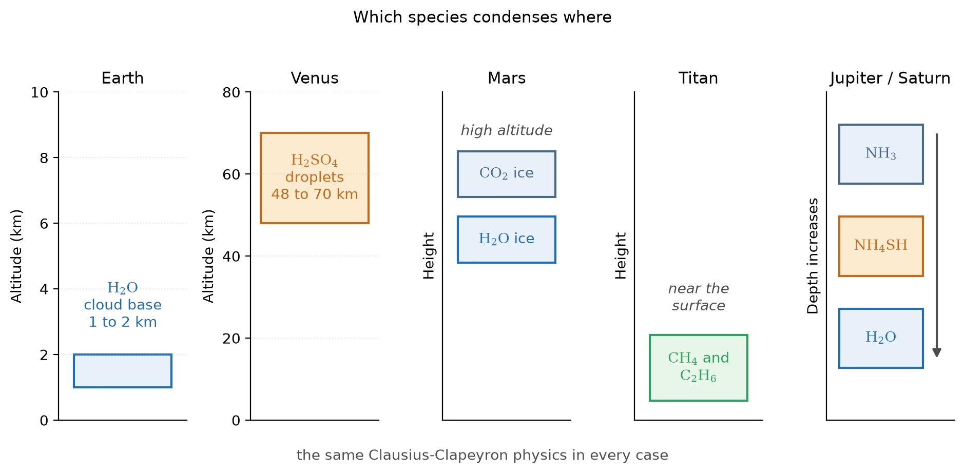
Fig. 6.4 Which species condenses where: Earth’s H\(_2\)O clouds with a base at 1 to 2 km, Venus’s H\(_2\)SO\(_4\) droplets at 48 to 70 km, CO\(_2\) and H\(_2\)O ice clouds at high altitude on Mars, CH\(_4\) and C\(_2\)H\(_6\) clouds in Titan’s lower troposphere, and the NH\(_3\), NH\(_4\)SH and H\(_2\)O decks at successively deeper levels on Jupiter and Saturn. The same Clausius-Clapeyron physics governs every case; only the species and its condensation temperature differ. Schematic; only the altitudes stated in the text are drawn to scale. Course-original figure.

6.2. Blackboard derivation: The Clausius-Clapeyron equation

Blackboard derivation: The Clausius-Clapeyron equation

Goal: Derive the exponential dependence of saturation vapour pressure on temperature from thermodynamic phase equilibrium, and apply the result to predict cloud condensation conditions across the solar system.

Setup: phase equilibrium.

Consider a substance (e.g., water) that exists in two phases: liquid and vapour. Along the coexistence curve in the \(P\)-\(T\) diagram (the line separating the liquid and vapour phases; see Fig. 6.6) the two phases are in thermodynamic equilibrium. This means the Gibbs free energy per unit mass is equal in both phases:

\[ g_{\ell}(T, P) = g_v(T, P) \]

where \(g_\ell\) and \(g_v\) are the specific Gibbs free energies of the liquid and vapour, respectively.

Fig. 6.5 shows the coexistence curve and the small step \((dT, dP)\) along it that the derivation takes.

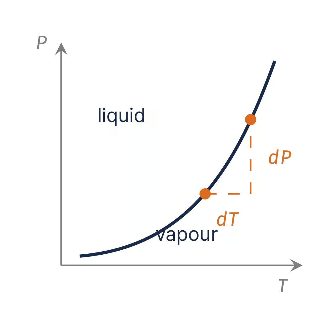
Fig. 6.5 Setup sketch of the board derivation of the Clausius-Clapeyron equation: the liquid-vapour coexistence curve in the \(P\)-\(T\) plane, with liquid above and vapour below, and a small step \(dT\), \(dP\) along the curve between two equilibrium states. Course-original figure.

Derivation.

If we move along the coexistence curve by an infinitesimal amount (\(\dd T\), \(\dd P\)), the Gibbs free energies must remain equal:

\[ \dd g_\ell = \dd g_v \]

From thermodynamics, \(\dd g = -s \, \dd T + v \, \dd P\), where \(s\) is the specific entropy and \(v\) is the specific volume. Therefore:

\[ -s_\ell \, \dd T + v_\ell \, \dd P = -s_v \, \dd T + v_v \, \dd P \]

Rearranging:

\[ (s_v - s_\ell) \, \dd T = (v_v - v_\ell) \, \dd P \]

\[ \dv{P}{T} = \frac{s_v - s_\ell}{v_v - v_\ell} = \frac{\Delta s}{\Delta v} \]

At the phase transition, the entropy change is related to the latent heat of vaporisation \(L_v\) (the energy required to convert one kilogram of liquid to vapour at constant temperature) by \(\Delta s = L_v / T\). Therefore:

\[ \dv{P_{\mathrm{sat}}}{T} = \frac{L_v}{T (v_v - v_\ell)} \]

This is the exact Clausius-Clapeyron relation. We now make two approximations:

1. The specific volume of the vapour is much larger than that of the liquid: \(v_v \gg v_\ell\), so \(v_v - v_\ell \approx v_v\).

2. The vapour behaves as an ideal gas: \(v_v = R_v T / P\), where \(R_v = R^* / M\) is the specific gas constant (\(R^* = 8.314\) J mol\(^{-1}\) K\(^{-1}\), \(M\) is the molar mass of the vapour).

Substituting:

\[ \dv{P_{\mathrm{sat}}}{T} = \frac{L_v \, P_{\mathrm{sat}}}{R_v \, T^2} \]

This is a separable ODE: \(\dd P / P = (L_v / R_v) \, \dd T / T^2\). Integrating from a reference state \((T_{\mathrm{ref}}, P_{\mathrm{ref}})\) to \((T, P_{\mathrm{sat}})\), with \(L_v\) treated as constant:

\[ \int_{P_{\mathrm{ref}}}^{P_{\mathrm{sat}}} \frac{\dd P'}{P'} = \frac{L_v}{R_v} \int_{T_{\mathrm{ref}}}^{T} \frac{\dd T'}{T'^2} \]

The left-hand integral gives \(\ln(P_{\mathrm{sat}}/P_{\mathrm{ref}})\). The right-hand integral gives \(\left[-1/T'\right]_{T_{\mathrm{ref}}}^{T} = -(1/T - 1/T_{\mathrm{ref}})\). Therefore:

\[ \ln \frac{P_{\mathrm{sat}}}{P_{\mathrm{ref}}} = -\frac{L_v}{R_v}\left(\frac{1}{T} - \frac{1}{T_{\mathrm{ref}}}\right) \]

Exponentiating both sides:

(6.1)\[ \boxed{P_{\mathrm{sat}}(T) = P_{\mathrm{ref}} \exp\!\left[-\frac{L_v}{R_v}\left(\frac{1}{T} - \frac{1}{T_{\mathrm{ref}}}\right)\right]} \]

This is the Clausius-Clapeyron equation. The saturation vapour pressure depends exponentially on temperature through the ratio \(L_v / R_v\), which has units of temperature and characterises the sensitivity of the phase transition.

Worked example: water on Earth.

For water vapour:

• \(L_v = 2.50 \times 10^6\) J kg\(^{-1}\) (latent heat of vaporisation at 0°C)

• \(M = 0.018\) kg mol\(^{-1}\), so \(R_v = 8.314 / 0.018 = 462\) J kg\(^{-1}\) K\(^{-1}\)

• Reference point: the triple point of water, \(T_{\mathrm{ref}} = 273\) K, \(P_{\mathrm{ref}} = 611\) Pa

The characteristic temperature scale is \(L_v / R_v = 2.50 \times 10^6 / 462 \approx 5400\) K. This large value (compared to typical atmospheric temperatures) is why \(P_{\mathrm{sat}}\) changes so rapidly with temperature.

At \(T = 293\) K (20°C):

\[\begin{split} \begin{aligned} P_{\mathrm{sat}} &= 611 \exp\!\left[-5400\left(\frac{1}{293} - \frac{1}{273}\right)\right] \\ &= 611 \exp(1.35) \approx 611 \times 3.86 \approx 2360 \text{ Pa} \approx 2.4 \text{ kPa} \end{aligned} \end{split}\]

The measured value is 2.3 kPa (excellent agreement). The small discrepancy arises because \(L_v\) decreases slightly with temperature (from \(2.50 \times 10^6\) J kg\(^{-1}\) at 0°C to \(2.26 \times 10^6\) J kg\(^{-1}\) at 100°C), which we neglected by treating \(L_v\) as constant.

Application: condensing species across the solar system.

The Clausius-Clapeyron equation applies to any vapour-to-liquid (or vapour-to-solid) transition. The following table lists the key condensing species in solar system atmospheres and their thermodynamic properties:

Species	\(L_v\) (kJ kg\(^{-1}\))	\(R_v\) (J kg\(^{-1}\) K\(^{-1}\))	\(L_v/R_v\) (K)	\(T_{\mathrm{cond}}\) (K)\(^*\)	Where it condenses
\(\mathrm{H_2O}\)	2500	462	5400	200–280	Earth, Mars
\(\mathrm{H_2SO_4}\)	540	85	6400	230–360	Venus
\(\mathrm{NH_3}\)	1370	488	2800	130–150	Jupiter, Saturn
\(\mathrm{CH_4}\)	510	519	980	80–90	Titan, Uranus, Neptune
\(\mathrm{CO_2}\)	571\(^\dagger\)	189	3020	100–150	Mars

\(^*\)Approximate condensation temperature at the pressure levels found in each planet’s atmosphere. \(^\dagger\)Latent heat of sublimation (solid \(\leftrightarrow\) vapour).

Data from [Catling and Kasting, 2017] and [de Pater and Lissauer, 2010].

The vertical sharpness of a cloud base follows from how fast \(P_{\mathrm{sat}}\) changes with altitude, \(\mathrm{d}\ln P_{\mathrm{sat}}/\mathrm{d}z = (L_v/R_v)\,\Gamma/T^2\), the product of the slope of the saturation curve and the lapse rate. Per kelvin the \(\mathrm{CH_4}\) curve near 90 K is even steeper than the \(\mathrm{H_2SO_4}\) curve near 350 K (0.12 against 0.05 K\(^{-1}\)), but Venus’s lapse rate of about 8 K km\(^{-1}\) compresses a factor-of-ten change of \(P_{\mathrm{sat}}\) into about 5 km, so its cloud base near 48 km is sharply defined and droplets that settle below it evaporate quickly. On Titan the weak gravity gives a lapse rate of only about 1.3 K km\(^{-1}\), the same factor of ten spans about 15 km, and methane clouds can form over a wide range of altitudes.

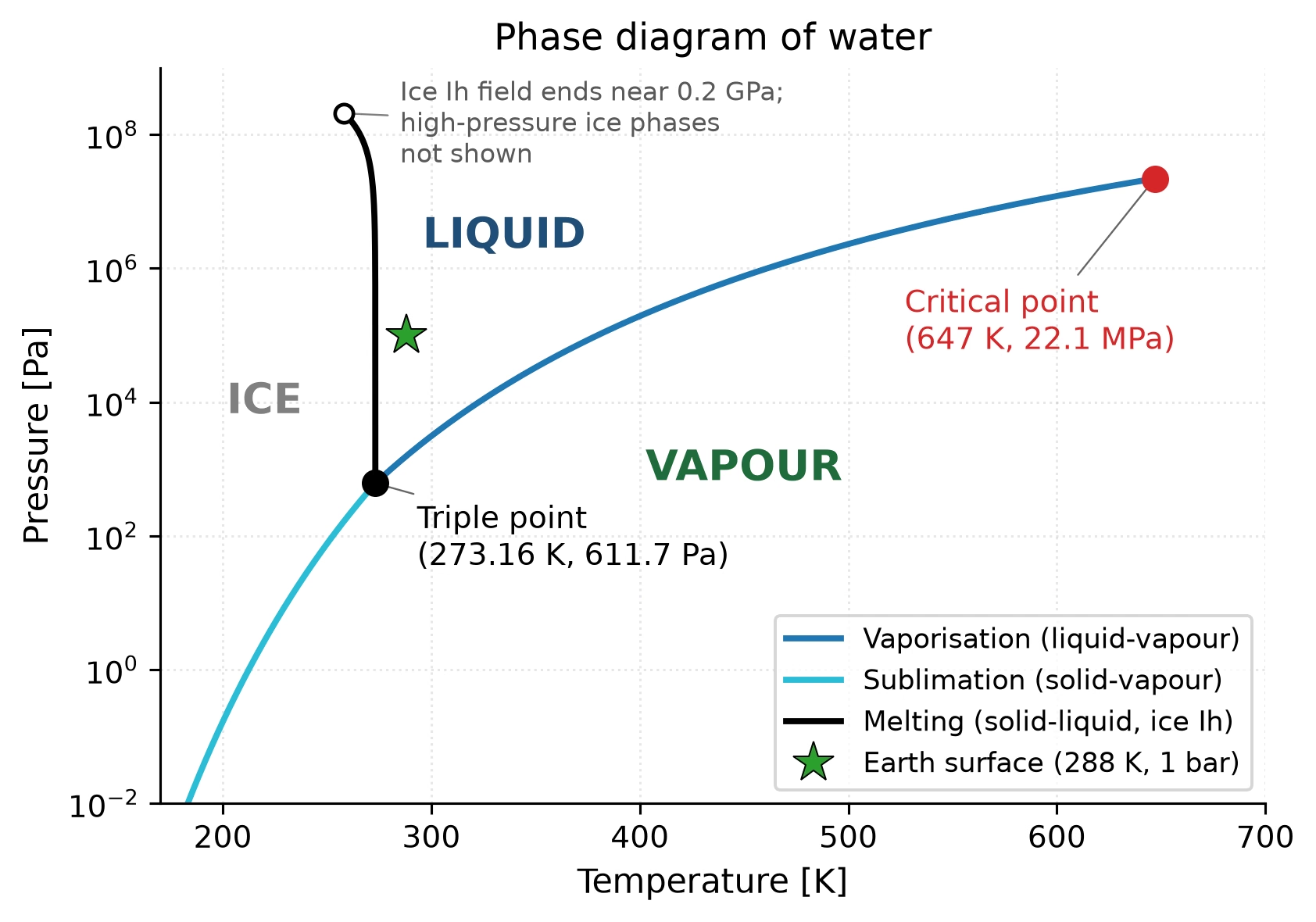
Fig. 6.6 Phase diagram of water in \(P\)-\(T\) space. The liquid-vapour coexistence curve (blue) is the integrated Clausius-Clapeyron relation (Eq. (6.1)); the solid-vapour (sublimation) curve (cyan) is the analogous Clausius-Clapeyron relation with the latent heat of sublimation; and the solid-liquid curve (black) has the anomalously negative slope characteristic of water (ice less dense than liquid). Because the integrated relation assumes a constant \(L_v\), the blue curve is drawn with an effective \(L_v = 2.29 \times 10^6\) J kg\(^{-1}\), the single value that makes it pass through both the triple point and the critical point; the worked example above instead uses the 0°C value \(L_v = 2.50 \times 10^6\) J kg\(^{-1}\) over a much narrower temperature range. The black curve is the melting curve of ice Ih only, and it stops where that field ends near 0.2 GPa; at higher pressure the slope reverses and denser ice phases take over, which the figure does not show. The triple point (273.16 K, 611.7 Pa) defines the unique state at which all three phases coexist. The critical point (647 K, 22.1 MPa) marks the end of the liquid-vapour distinction. Earth’s surface (288 K, 1 bar) sits well within the liquid-vapour stability field, which is why liquid water is the dominant condensable on the planet. The blackboard derivation in this lecture integrates the Clausius-Clapeyron equation along the blue curve. Course-original figure.

6.3. Clouds across the solar system

Every planet and moon with a substantial atmosphere has clouds, but the condensing species and the cloud structure vary enormously. Here we survey the major cloud systems in our solar system [Sánchez-Lavega, 2011].

6.3.1. Venus: sulfuric acid clouds

Venus is permanently shrouded in thick clouds that completely obscure the surface at visible wavelengths. These clouds are composed of \(\mathrm{H_2SO_4}\) (sulfuric acid) droplets and extend from \(\sim\)48 km to \(\sim\)70 km altitude, spanning a temperature range of roughly 360–230 K between cloud base and cloud top [Catling and Kasting, 2017].

The cloud deck completely obscures the surface in visible light; UV imaging reveals the banded pattern produced by super-rotation, the clouds circling the planet far faster than the solid surface rotates beneath them (Fig. 6.7). The sulfuric acid is produced by photochemistry in the upper atmosphere:

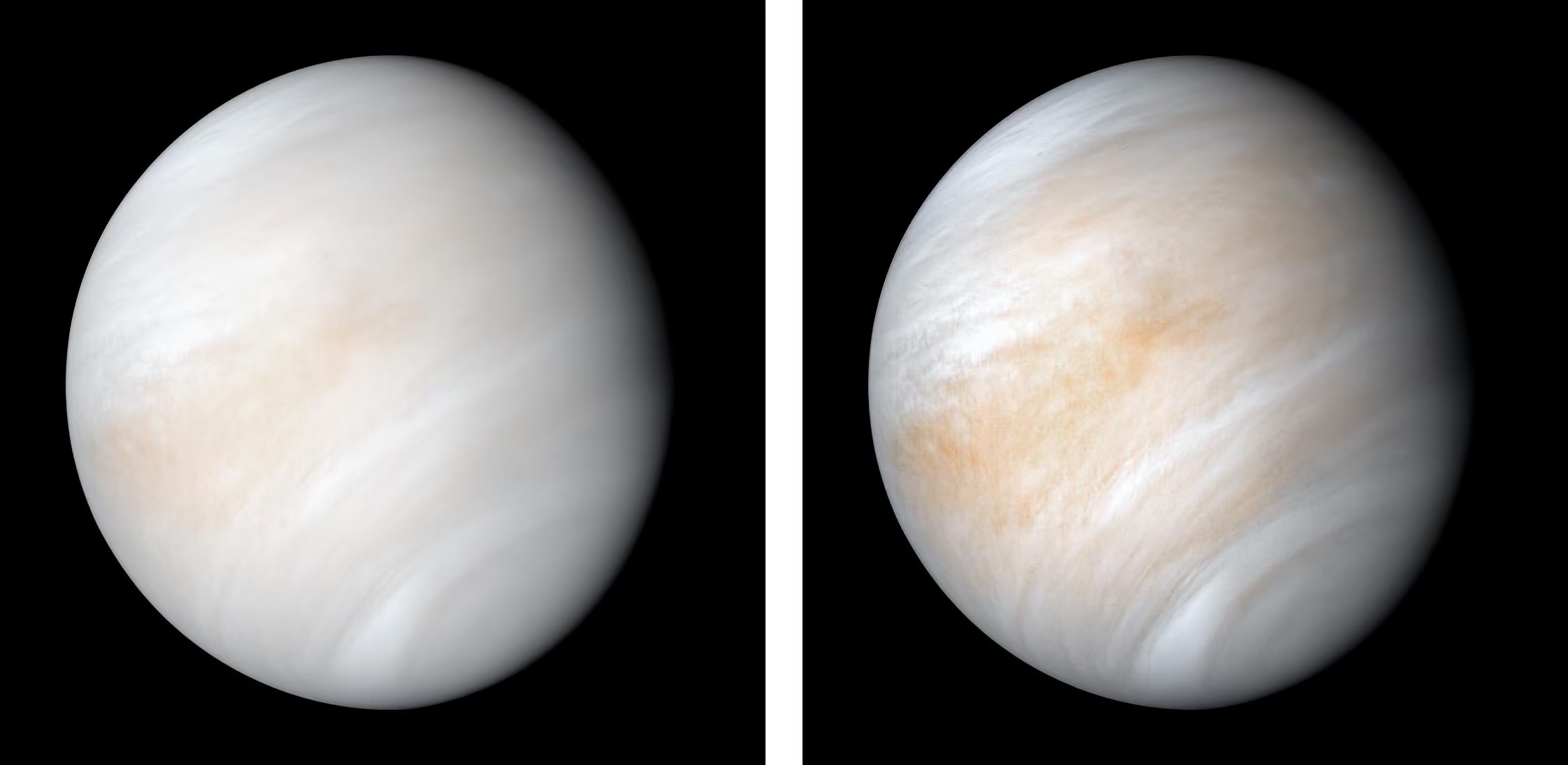
Fig. 6.7 Venus imaged by the Mariner 10 spacecraft in February 1974, using a false-colour composite of orange and ultraviolet filters to reveal the banded cloud structure driven by atmospheric super-rotation. The \(\mathrm{H_2SO_4}\) cloud deck extends from \(\sim\)48 to \(\sim\)70 km altitude and completely obscures the surface. Credit: NASA/JPL-Caltech, public domain.

\[ \mathrm{SO_2} + \mathrm{O} \longrightarrow \mathrm{SO_3}, \qquad \mathrm{SO_3} + \mathrm{H_2O} \longrightarrow \mathrm{H_2SO_4} \]

where the atomic oxygen comes from ultraviolet photolysis of \(\mathrm{CO_2}\) high in the atmosphere, and the \(\mathrm{SO_2}\) is supplied by volcanic outgassing. The sub-cloud haze and the unidentified upper-cloud UV absorber, which takes up roughly half of the incident solar UV flux, remain open questions, while Venus’s vertical thermal structure is shown in Fig. 6.8.

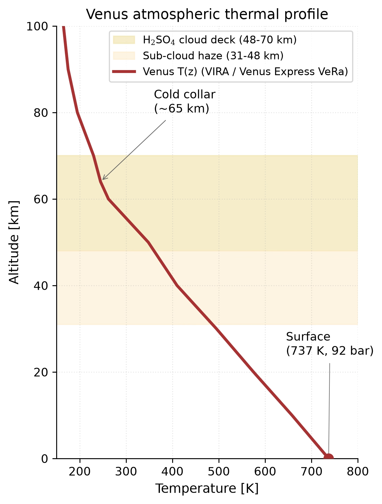
Fig. 6.8 Venus thermal structure from the surface (737 K, 92 bar) to 100 km altitude, based on the Venus International Reference Atmosphere and the Venus Express radio-science experiment [Tellmann et al., 2009]. The \(\mathrm{H_2SO_4}\) cloud deck (yellow band, 48-70 km) sits where the temperature traverses \(\sim\)230-360 K between cloud top and cloud base, within the thermodynamic stability field of concentrated sulfuric acid droplets; the sub-cloud haze (peach band, 31-48 km) lies just below. The marker near 65 km locates the cold collar; this mid-latitude profile falls monotonically, and the temperature inversion that the VeRa retrievals show there at high latitudes (\(\sim\)65-75°) is not drawn. Course-original figure.

6.3.2. Mars: dust and ice clouds

Mars’s thin atmosphere (\(\sim\)6 mbar surface pressure) supports high-altitude \(\mathrm{CO_2}\) ice clouds and lower \(\mathrm{H_2O}\) ice clouds nucleated on wind-lofted mineral dust. An orbital view of such water-ice clouds draped across the Tharsis volcanoes is shown in Fig. 6.9.

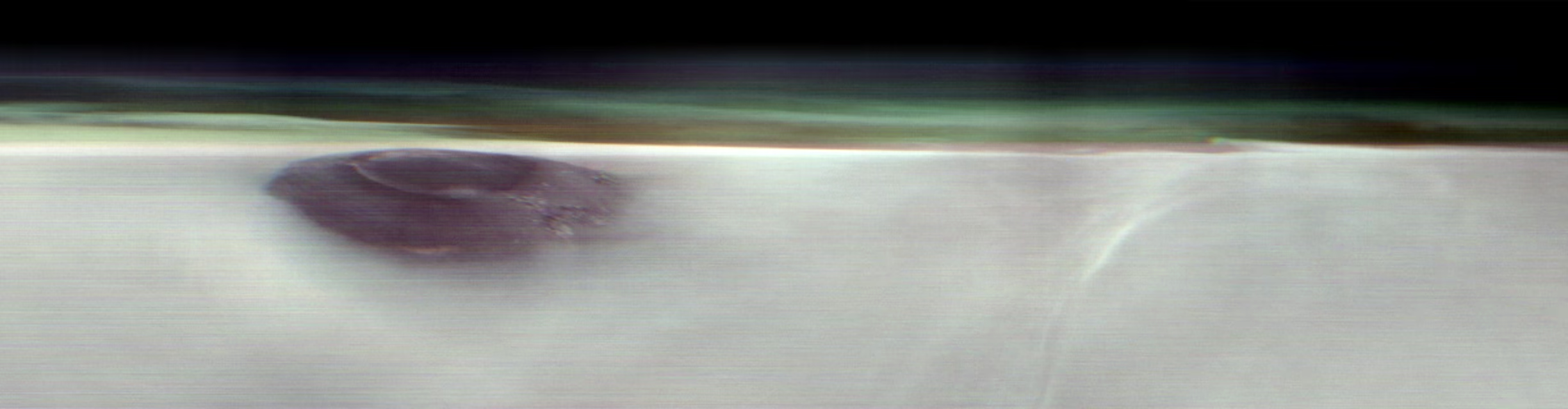
Fig. 6.9 Water-ice clouds over the Tharsis region of Mars near dawn, viewed along the limb from orbit. The dark peak breaking through the bright cloud canopy (left of centre) is the summit of the shield volcano Arsia Mons. These are the \(\mathrm{H_2O}\) ice clouds described above. They form when air cools as it rises over the high volcanic terrain, and again near the equator when the seasonal aphelion cloud belt develops. The panorama was recorded by the THEMIS instrument on NASA’s Mars Odyssey orbiter on 2 May 2025. Credit: NASA/JPL-Caltech/ASU, public domain.

6.3.3. Titan: methane rain

Saturn’s moon Titan hosts the only known active hydrological cycle beyond Earth, but with \(\mathrm{CH_4}\) (methane) playing the role of water. Titan’s surface temperature (\(\sim\)94 K) and pressure (\(\sim\)1.5 bar) place it near the triple point of methane, enabling liquid methane on the surface (lakes and seas), methane clouds in the troposphere, and methane rain [de Pater and Lissauer, 2010]. Streaks of these tropospheric methane clouds appear in Fig. 6.10.

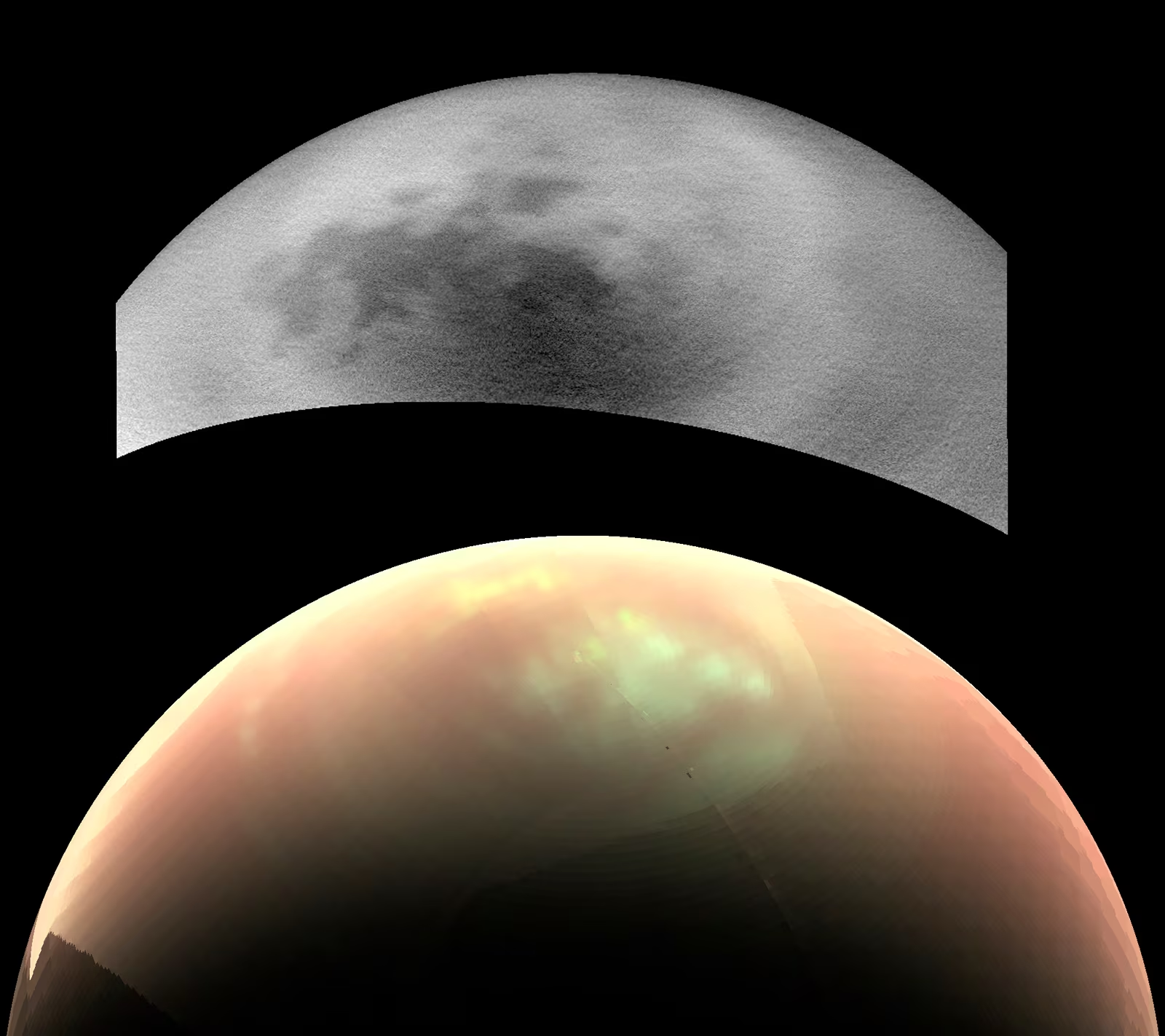
Fig. 6.10 Methane-ethane clouds at Titan’s mid-southern latitudes captured by the Cassini Imaging Science Subsystem in the 938 nm methane window. The bright streaks near the limb are tropospheric clouds organised along the local zonal (east-west) wind, which shows that Titan supports an active condensation cycle of the same Clausius-Clapeyron physics described in this lecture, but with \(\mathrm{CH_4}\) replacing \(\mathrm{H_2O}\) at \(T \approx 90\) K. Credit: NASA/JPL-Caltech/Space Science Institute, public domain.

Titan’s clouds are mostly \(\mathrm{CH_4}\) (condensing at \(\sim\)8–30 km altitude) with some \(\mathrm{C_2H_6}\) (ethane); infrequent but intense methane rain feeds surface lakes and river channels [Stofan et al., 2007] (Lecture 11). The radar-dark polar lakes and seas formed by this runoff are shown in Fig. 6.11.

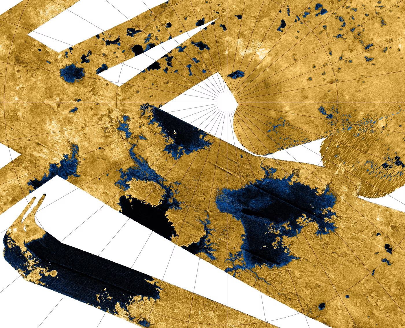
Fig. 6.11 Titan’s north polar lake district imaged by the Cassini RADAR instrument. The first detection [Stofan et al., 2007] resolved more than 75 radar-dark lake-like patches poleward of \(\sim\)70°N latitude, ranging from 3 to over 70 km across; subsequent Cassini RADAR coverage of the high-latitude seas mapped the three largest maria: Kraken Mare, Ligeia Mare, and Punga Mare, each hundreds of kilometres across, here interpreted as standing bodies of liquid methane and ethane. Together with the methane-cloud observations and inferred rainfall, these lakes constitute the visible surface end of the only active hydrocarbon hydrological cycle in the solar system. Credit: NASA/JPL-Caltech/ASI/USGS, public domain.

6.3.4. Giant planets: layered cloud structure

The hydrogen-dominated atmospheres of Jupiter and Saturn host a vertically layered cloud structure, predicted by the Clausius-Clapeyron equation applied to each condensing species at the temperature and pressure where it reaches saturation [de Pater and Lissauer, 2010]:

1. \(\mathrm{NH_3}\) ice (topmost layer): condensing at \(T \sim 130\)–150 K, \(P \sim 0.5\)–1 bar. These are the clouds we see in visible light: the white and coloured bands of Jupiter.

2. \(\mathrm{NH_4SH}\) (ammonium hydrosulfide): condensing at \(T \sim 200\)–240 K, \(P \sim 2\)–3 bar. Formed by the reaction \(\mathrm{NH_3} + \mathrm{H_2S} \to \mathrm{NH_4SH}\).

3. \(\mathrm{H_2O}\) ice and liquid (deepest layer): condensing at \(T \sim 270\)–300 K, \(P \sim 5\)–7 bar. These deep water clouds are difficult to observe directly but are thought to play a critical role in powering Jupiter’s weather through latent heat release.

The vertical layering of these three cloud decks is sketched in Fig. 6.12.

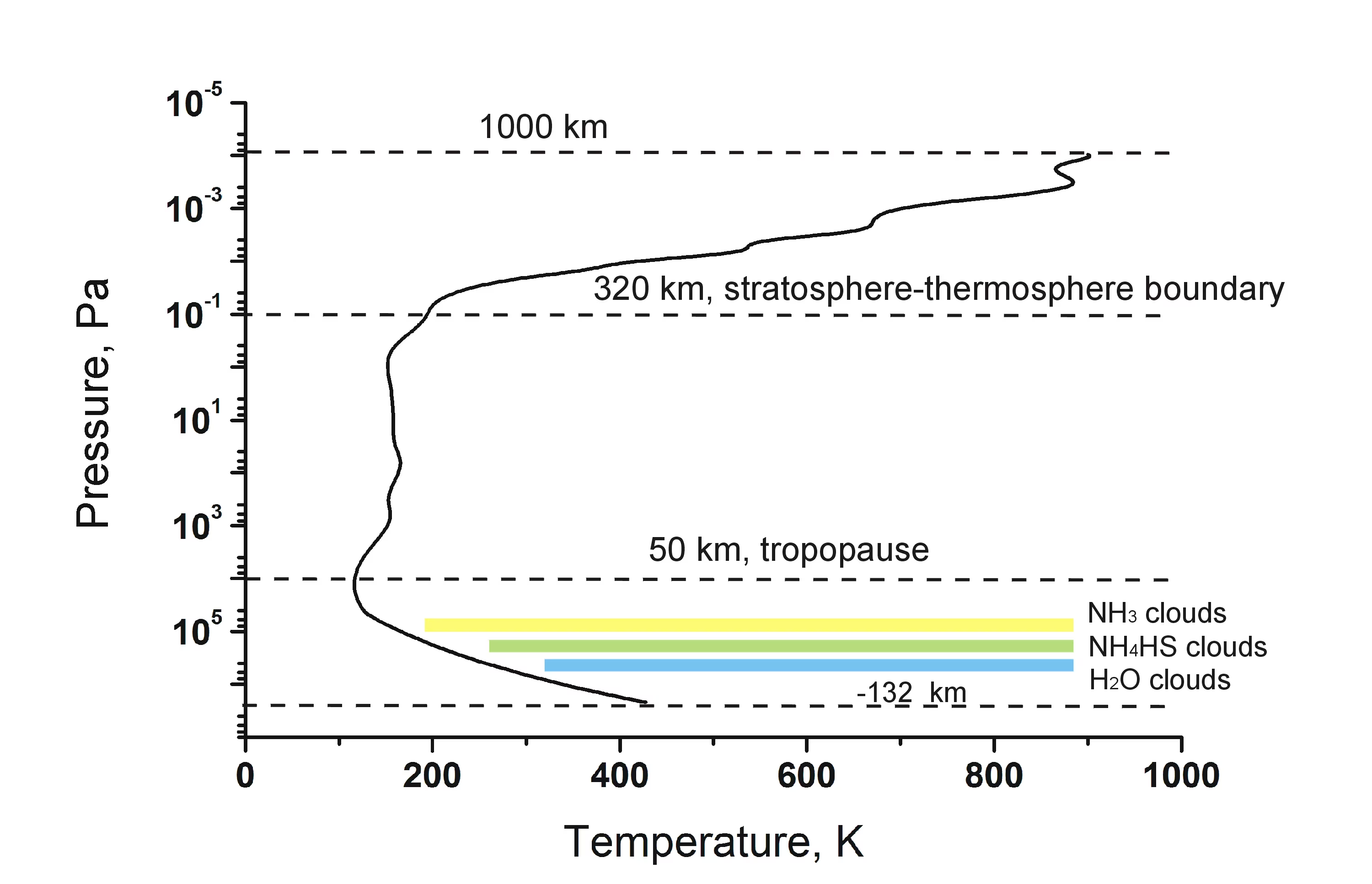
Fig. 6.12 Temperature–pressure profile of Jupiter’s atmosphere, showing the three main cloud layers: ammonia (\(\mathrm{NH_3}\)) ice at the top (\(\sim\)1 bar), ammonium hydrosulfide (\(\mathrm{NH_4SH}\)) in the middle (\(\sim\)2–3 bar), and water (\(\mathrm{H_2O}\)) at the deepest level (\(\sim\)5–7 bar). The tropopause, the boundary where temperature stops falling with altitude and convective mixing gives way to a stably stratified layer above, sits at \(\sim\)50 km, and the stratosphere-thermosphere boundary at \(\sim\)320 km is marked as well. Each cloud layer sits at the pressure level where the temperature profile crosses the condensation temperature of that species (the saturation curves themselves are not drawn). Credit: Wikimedia Commons, CC BY-SA 3.0.

The visible cloud-band morphology produced by these layers across Jupiter’s full disk is shown in Fig. 6.13.

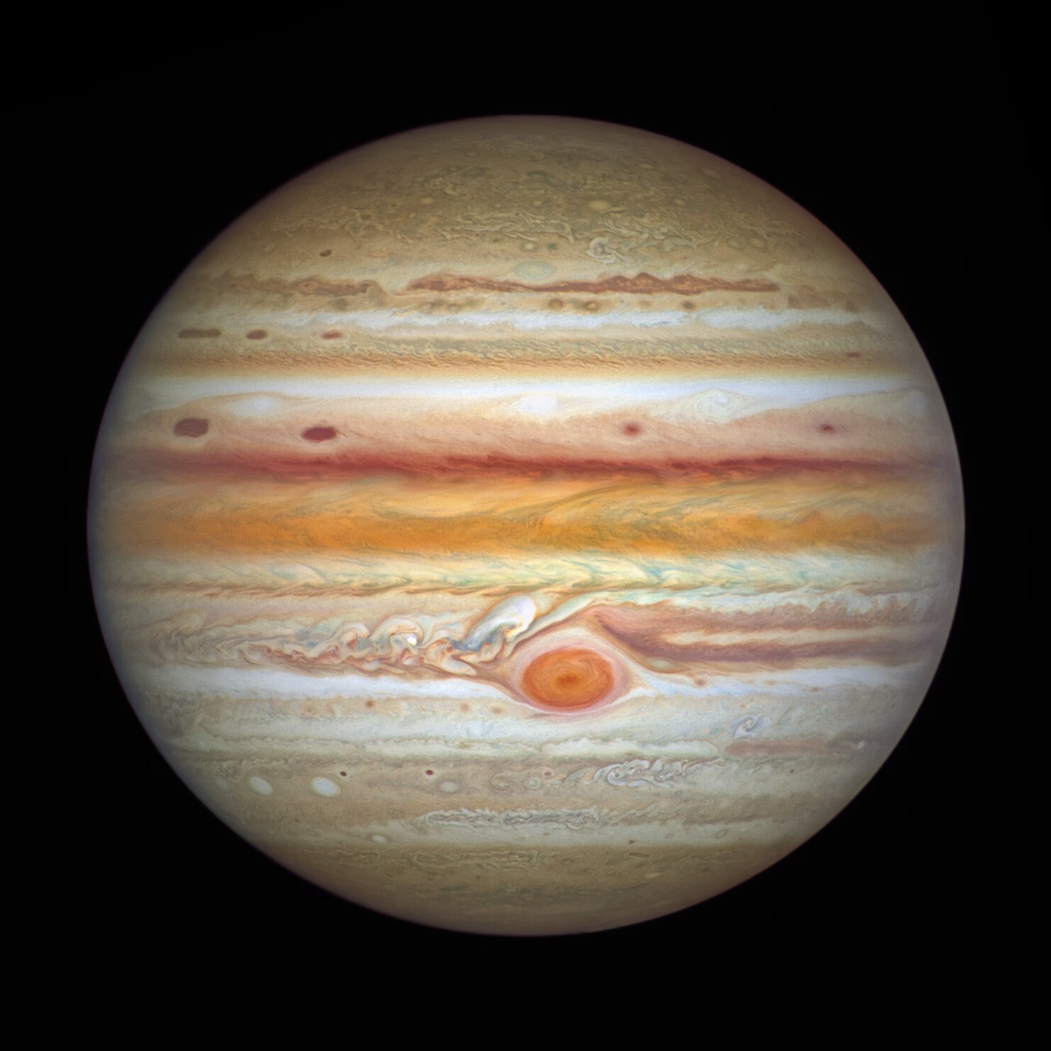
Fig. 6.13 Full-disk portrait of Jupiter from the Hubble Space Telescope, observed on 4 September 2021 as part of the Outer Planets Atmospheres Legacy (OPAL) programme. The banded structure is clear: light zones (rising air topped by high \(\mathrm{NH_3}\)-ice clouds) alternate with dark belts (sinking air that exposes the deeper \(\mathrm{NH_4SH}\) layer). The Great Red Spot appears at \(\sim\)22°S, just south of the dark South Equatorial Belt. These narrow latitudinal contrasts trace the alternating zonal-jet system that long-term Hubble programmes have monitored for over a decade [Wong et al., 2020]; the jets extend to \(\sim \pm 60^\circ\) and are summarised quantitatively below. Credit: NASA, ESA, A. Simon (GSFC), M. H. Wong (UC Berkeley), and the OPAL team; ESA/Hubble, CC BY 4.0.

The ice giants Uranus and Neptune have a different cloud hierarchy topped by \(\mathrm{CH_4}\) ice at \(T \sim 80\) K with deeper \(\mathrm{H_2S}\), \(\mathrm{NH_4SH}\), and \(\mathrm{H_2O}\) layers.

6.4. Atmospheric dynamics

Atmospheres are not static: they are vast heat engines driven by uneven heating. The equator receives more solar energy per unit area than the poles, creating a temperature gradient that drives global-scale circulation patterns. How the atmosphere redistributes this heat depends on the planet’s rotation rate, size, and atmospheric properties [Sánchez-Lavega, 2011].

6.4.1. The Hadley cell

The simplest atmospheric circulation pattern, first described by George Hadley in 1735, works as follows:

1. Intense solar heating at the equator warms the surface and the air above it.

2. Warm, buoyant air rises at the equator, creating a low-pressure zone (the Intertropical Convergence Zone, ITCZ).

3. At altitude, the air flows poleward (toward higher latitudes).

4. As it moves poleward, it cools radiatively, becomes denser, and sinks at \(\sim\)30° latitude (the subtropics), creating high-pressure zones (where Earth’s great deserts are located).

5. At the surface, air flows back toward the equator to replace the rising air: these return flows are the trade winds.

This loop is the Hadley cell (Fig. 6.14). It is the dominant circulation pattern in the tropics on Earth and the primary mechanism for transporting heat from the equator toward the poles.

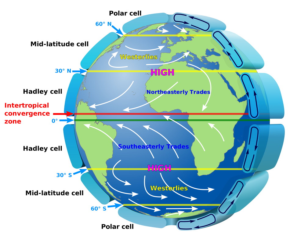
Fig. 6.14 Schematic of Earth’s atmospheric circulation, showing the three-cell structure in each hemisphere: the Hadley cell (equator to \(\sim\)30°), the Ferrel cell (\(\sim\)30° to \(\sim\)60°, labelled “mid-latitude cell” here), and the polar cell (\(\sim\)60° to the pole). The northeasterly and southeasterly trade winds and the westerlies are labelled as the surface expression of these cells, together with the intertropical convergence zone at the equator and the subtropical high-pressure belt. The Coriolis effect deflects the winds to the right in the Northern Hemisphere and to the left in the Southern Hemisphere. Credit: Wikimedia Commons, public domain.

6.4.2. The Coriolis effect

On a rotating planet, air that moves in a straight line (as seen from an inertial frame) appears to be deflected as seen from the rotating surface. This apparent deflection is the Coriolis effect: moving air is deflected to the right in the Northern Hemisphere and to the left in the Southern Hemisphere.

The magnitude of the Coriolis acceleration depends on the planet’s angular rotation rate \(\Omega\) and the latitude \(\phi\) through the Coriolis parameter:

\[ f = 2\Omega \sin\phi \]

For Earth, \(\Omega = 7.29 \times 10^{-5}\) rad s\(^{-1}\) (sidereal rotation rate). At mid-latitudes (\(\phi = 45°\)), \(f \approx 1.03 \times 10^{-4}\) s\(^{-1}\). At the equator (\(\phi = 0°\)), \(f = 0\): the Coriolis effect vanishes. The kinematic origin of the deflection is shown in Fig. 6.15.

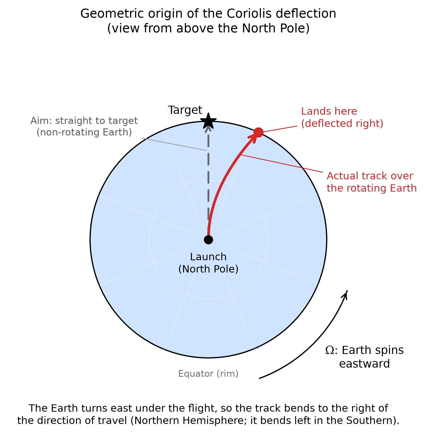
Fig. 6.15 Geometric origin of the Coriolis deflection, viewed from above the rotating planet’s north pole (centre), with the equator at the rim. A projectile launched from the pole has no eastward velocity, so on a non-rotating planet it would travel straight to its target (dashed line). Because the planet turns east under the flight with angular velocity \(\Omega\), the track over the ground curves to the right of the direction of travel in the Northern Hemisphere (red curve) and lands to the right of the target. Launching from the pole isolates the effect: the aim is a straight radial line, and the deflection comes entirely from the ground rotating beneath the flight. The strength of the deflection is set by the Coriolis parameter \(f = 2 \Omega \sin \phi\): it vanishes at the equator and is strongest at the poles, and in the Southern Hemisphere the deflection is mirrored to the left. The deflection angle shown is exaggerated for clarity. Course-original figure.

6.4.3. The Rossby number

Whether rotation significantly influences a particular atmospheric flow depends on the Rossby number, which compares the inertial acceleration to the Coriolis acceleration:

\[ \mathrm{Ro} = \frac{U}{f L} \]

where \(U\) is the characteristic wind speed and \(L\) is the characteristic horizontal length scale of the flow.

• \(\mathrm{Ro} \ll 1\): Rotation dominates; the flow is strongly influenced by the Coriolis effect. This applies to large-scale atmospheric and oceanic circulation on Earth (e.g., \(U \sim 10\) m s\(^{-1}\), \(L \sim 1000\) km \(\Rightarrow \mathrm{Ro} \sim 0.1\)).

• \(\mathrm{Ro} \gg 1\): Rotation is unimportant; the flow is governed by pressure gradients and friction. This applies to small-scale phenomena like tornadoes and dust devils.

Fig. 6.16 sorts these flows on the plane of length scale against wind speed.

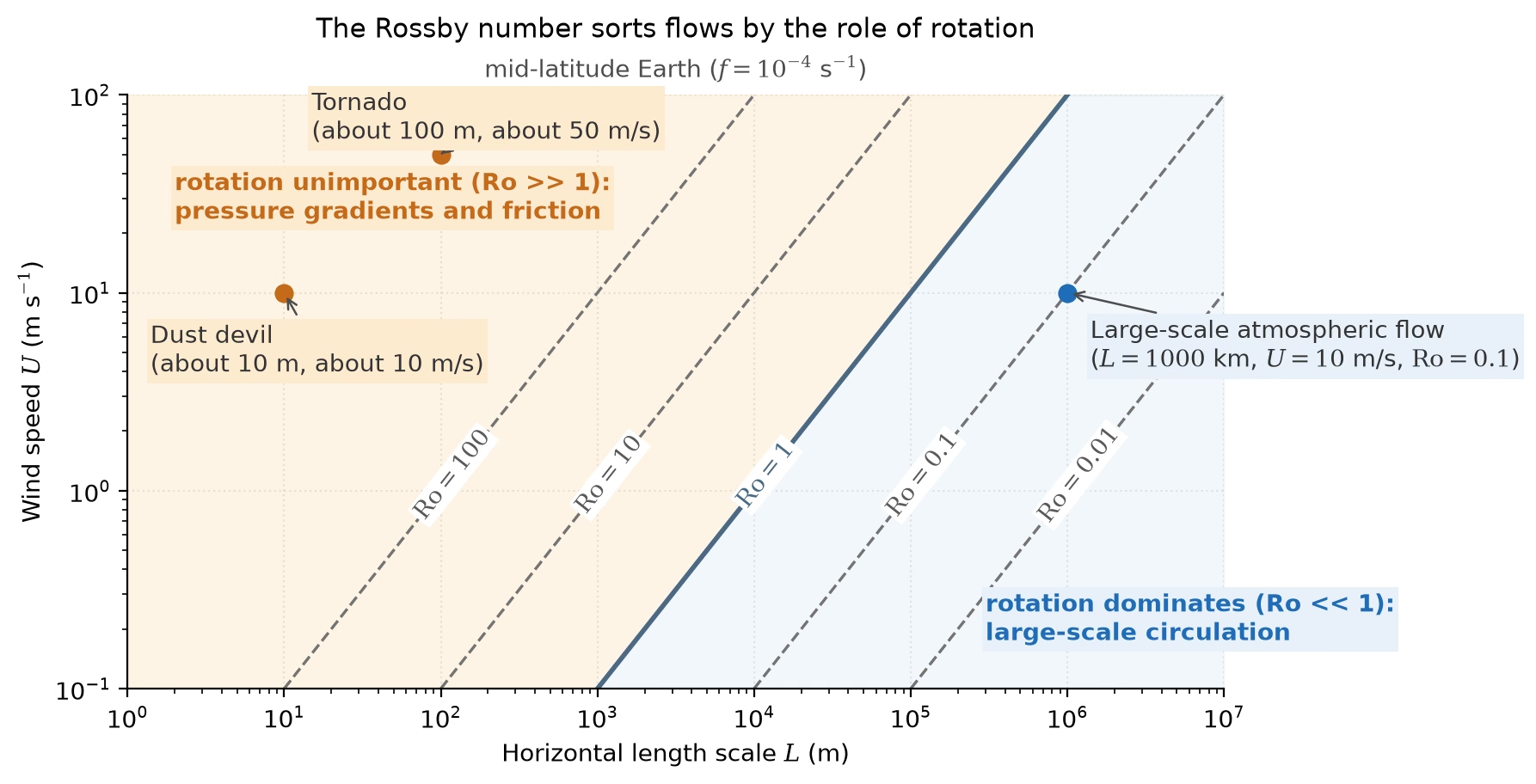
Fig. 6.16 Flow regimes sorted by the Rossby number \(\mathrm{Ro} = U/(fL)\) for mid-latitude Earth (\(f = 10^{-4}\) s\(^{-1}\)): lines of constant \(\mathrm{Ro}\) on the plane of horizontal length scale against wind speed. Large-scale circulation (\(U \sim 10\) m s\(^{-1}\), \(L \sim 1000\) km, \(\mathrm{Ro} \sim 0.1\)) lies in the rotation-dominated region; a dust devil (about 10 m, about 10 m s\(^{-1}\)) and a tornado (about 100 m, about 50 m s\(^{-1}\)) lie far inside the region where pressure gradients and friction govern the flow. The dust devil and tornado sizes are order-of-magnitude examples. Course-original figure.

6.4.4. Circulation cells and rotation rate

The number of circulation cells depends critically on the planet’s rotation rate [de Pater and Lissauer, 2010]:

• Slowly rotating planets (Venus, Titan): A single Hadley cell extends from equator to pole in each hemisphere. Venus has one giant Hadley cell per hemisphere despite being nearly the same size as Earth, because its slow rotation (243-day period) gives very small Coriolis forces (\(\mathrm{Ro} \gg 1\) for large-scale flows).

• Moderately rotating planets (Earth): The Hadley cell extends to \(\sim\)30° latitude, where the Coriolis deflection becomes strong enough to break the cell. Two additional cells form at higher latitudes: the Ferrel cell (mid-latitudes, driven indirectly by the Hadley and polar cells) and the polar cell. Earth has three cells per hemisphere.

• Rapidly rotating planets (Jupiter, Saturn): Many alternating cells form, producing the characteristic banded structure of alternating light zones (rising air, high clouds) and dark belts (sinking air, deeper cloud exposure). Jupiter and Saturn each show many alternating jets per hemisphere, extending to roughly \(\pm 60^\circ\) latitude.

The transition between regimes is governed by the ratio of the planet’s rotation timescale to the advective timescale across the planet. When rotation is fast compared to the time for air to flow from equator to pole, the flow breaks up into multiple cells. The resulting overturning circulation for a moderately rotating planet like Earth, showing the Hadley, Ferrel, and polar cells in latitude and altitude, is illustrated by the meridional streamfunction in Fig. 6.17.

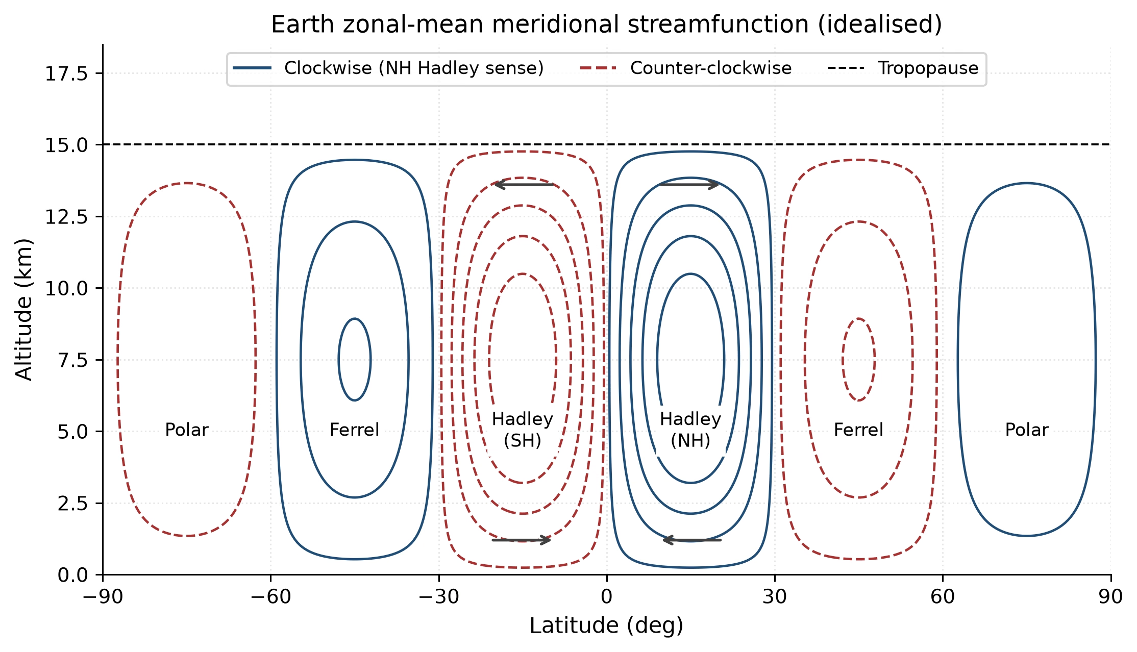
Fig. 6.17 Idealised zonal-mean meridional streamfunction of Earth’s troposphere, plotted as latitude versus altitude. Solid blue contours mark clockwise overturning in this latitude-altitude view, the sense of the Northern-Hemisphere Hadley cell (rising at the equator, poleward aloft, sinking near 30°); dashed red contours mark counter-clockwise overturning, arrows on the two Hadley cells show the flow direction, and the dashed black line indicates the tropopause. The two thermally direct Hadley cells flank the equator from the surface to \(\sim\)15 km, the indirect Ferrel cells lie between \(\sim\)30° and \(\sim\)60° in each hemisphere, and the weak polar cells sit poleward of \(\sim\)60°. The cell structure follows the Held and Hou [1980] axisymmetric theory of nearly inviscid atmospheres. Course-original figure.

6.5. Geostrophic balance and jet streams

6.5.1. Geostrophic balance

At large scales (low Rossby number), the atmosphere reaches a steady state in which the Coriolis force balances the pressure gradient force. This balance is called geostrophic balance and is the dominant force balance for large-scale weather systems on Earth and the banded circulations of the giant planets [Pierrehumbert, 2010].

In vector form, geostrophic balance reads:

(6.2)\[ f \hat{k} \times \mathbf{v}_g = -\frac{1}{\rho} \nabla P \]

where \(\hat{k}\) is the local vertical unit vector (normal to the surface), \(\mathbf{v}_g\) is the geostrophic wind, \(\rho\) is the air density, and \(\nabla P\) is the horizontal pressure gradient.

The key consequence is that the geostrophic wind blows parallel to isobars (lines of constant pressure), not from high to low pressure as one might naively expect. In the Northern Hemisphere, the wind blows with low pressure to its left; in the Southern Hemisphere, low pressure is to the right. This is why large-scale weather systems (cyclones and anticyclones) rotate around pressure centres rather than flowing directly toward them.

The vector force balance, with the wind blowing parallel to isobars rather than down the pressure gradient, is shown in Fig. 6.18. In scalar form, the geostrophic wind components are:

\[ u_g = -\frac{1}{f\rho} \pdv{P}{y}, \qquad v_g = \frac{1}{f\rho} \pdv{P}{x} \]

where \(x\) and \(y\) are the eastward and northward directions, respectively.

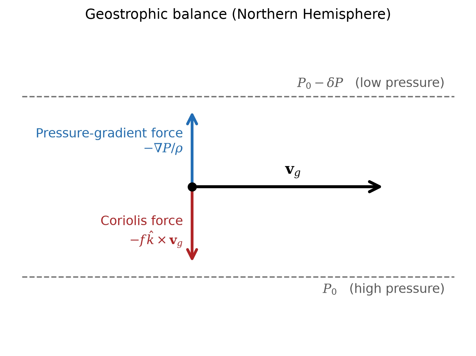
Fig. 6.18 Geostrophic balance between the horizontal pressure-gradient force (\(-\nabla P / \rho\), blue arrow) and the Coriolis force (\(-f \hat{k} \times \mathbf{v}_g\), red arrow), giving a wind \(\mathbf{v}_g\) that blows parallel to the isobars rather than down the pressure gradient. In the Northern Hemisphere the balanced wind keeps low pressure to its left. This is the dominant balance for large-scale flow on Earth and the giant planets (discussed below) where the Rossby number is small. Course-original figure.

6.5.2. Jet streams

Jet streams are narrow bands of fast-moving air (\(\sim\)30–70 m s\(^{-1}\) on Earth) that form at the boundaries between circulation cells, where horizontal temperature gradients are strongest. Their existence is a direct consequence of the thermal wind relation, which connects vertical wind shear to horizontal temperature gradients:

\[ \pdv{\mathbf{v}_g}{z} \propto \hat{k} \times \nabla T \]

Where the temperature gradient between the warm tropics and the cold poles is steepest (at \(\sim\)30° and \(\sim\)60° latitude on Earth), the wind speed increases with altitude, producing the subtropical and polar jet streams. These jet streams steer weather systems across the planet and are critical for understanding weather patterns (Fig. 6.19).

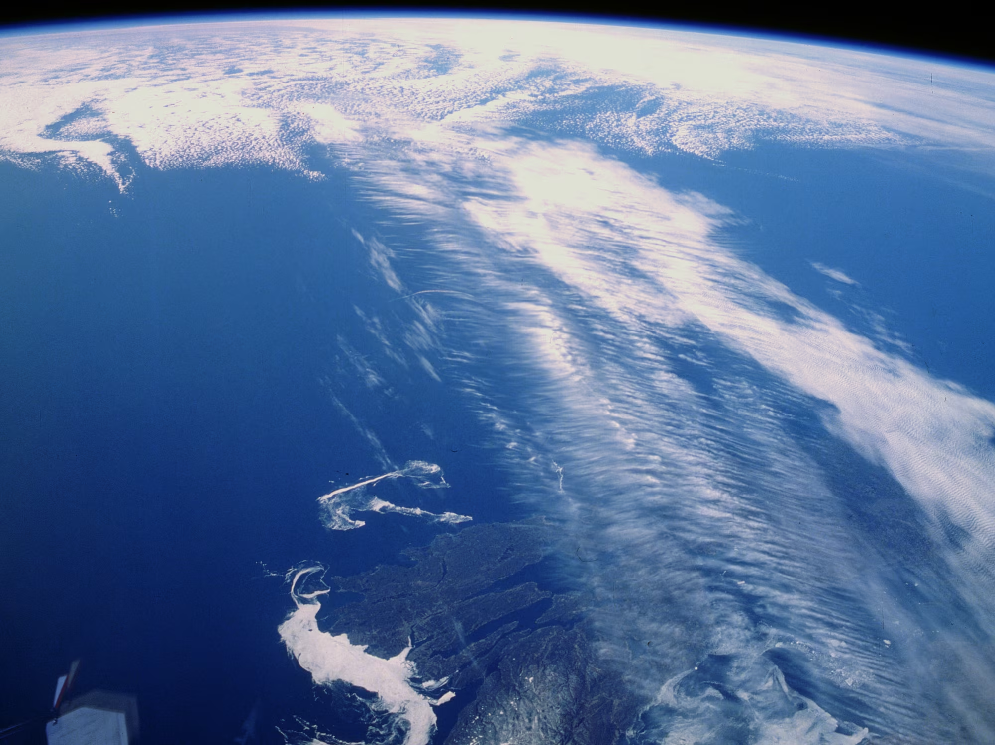
Fig. 6.19 An Earth-from-orbit astronaut photograph showing long cirrus filaments streaked across the limb above a dark sea and coastline. Such aligned cirrus bands trace the upper-tropospheric jet core at \(\sim\)200-250 hPa, where horizontal temperature gradients drive thermal-wind shear of order 30-70 m s\(^{-1}\); weather systems are steered along the layer in which these filaments form. Credit: NASA astronaut photograph, Johnson Space Center, public domain.

6.5.3. Giant planet banding

On Jupiter and Saturn, the alternating light and dark bands (the zones and belts) correspond to regions of rising and sinking air bounded by strong zonal jets (Fig. 6.20), which extend deep into the planetary interior as revealed by Juno gravity measurements (Lecture 11) [Kaspi et al., 2018].

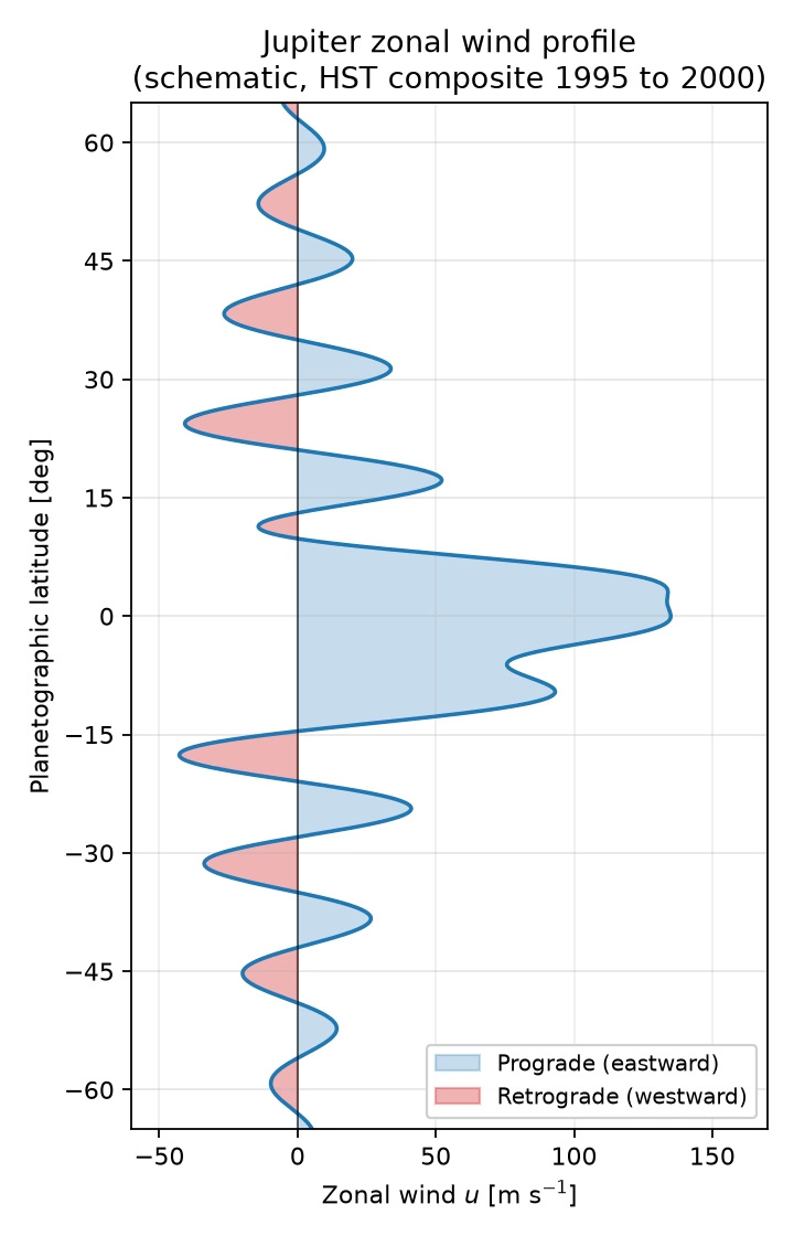
Fig. 6.20 Jupiter’s cloud-top zonal wind profile \(u(\phi)\), schematic representation of the HST composite (1995-2000) of García-Melendo and Sánchez-Lavega [2001]. A ladder of narrow prograde (eastward, blue) and retrograde (westward, red) jets is stacked from the broad equatorial superrotating jet at the centre out to \(\sim\)60° latitude (the schematic resolves only the principal jets to keep the figure legible). The jets coincide with the boundaries between bright zones and dark belts, and Juno gravity measurements yield a best-fit e-folding decay depth (the depth over which the jet strength falls by a factor of \(1/e\)) of \(\sim\)1800 km, with the full uncertainty range spanning \(\sim\)1000–3000 km into the molecular envelope [Kaspi et al., 2018].

6.6. Weather and storms across the solar system

Planets and moons exhibit a stunning variety of weather phenomena, from gentle breezes to apocalyptic storms. Here we survey the highlights.

6.6.1. Mars: dust storms and seasonal cycles

Mars experiences dramatic weather driven by a seasonal \(\mathrm{CO_2}\) cycle where polar cap condensation and sublimation swing atmospheric mass by \(\sim\)25–30% (from \(\sim\)5 to \(\sim\)7 mbar), while positive radiative feedback from wind-lofted mineral dust triggers global dust storms (Lecture 10) [Catling and Kasting, 2017]. The resulting global obscuration is shown for the 2018 event in Fig. 6.21.

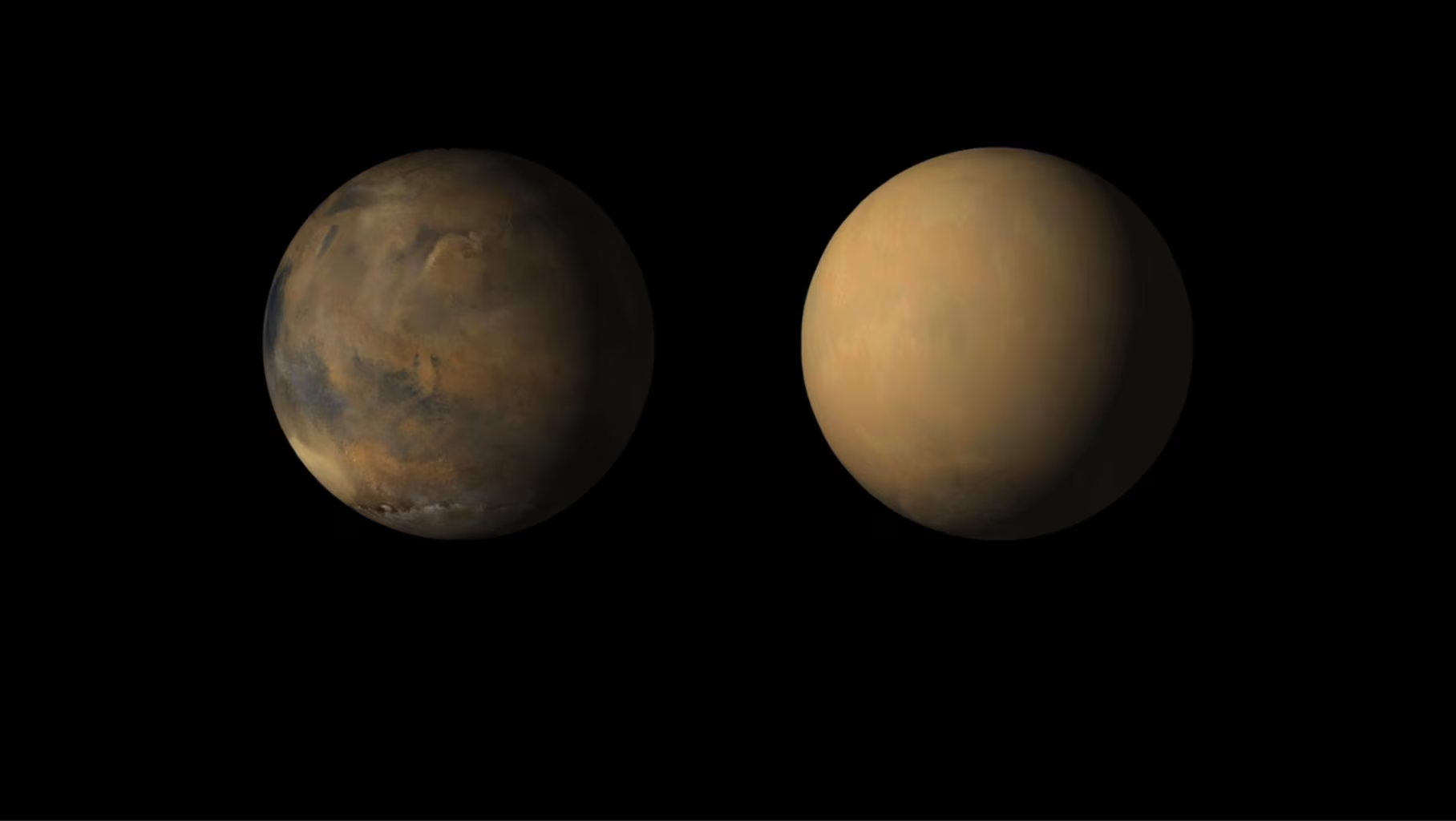
Fig. 6.21 Mars before and during the 2018 global dust storm, as imaged by the Mars Reconnaissance Orbiter. The left panel shows clear atmospheric conditions with surface features visible; the right panel shows the planet almost completely obscured by wind-lofted mineral dust. The storm ultimately ended the Opportunity rover’s 15-year mission by blocking sunlight to its solar panels. Credit: NASA/JPL-Caltech/MSSS, public domain.

6.6.2. Venus: super-rotation

Venus presents one of the great puzzles of atmospheric dynamics: its atmosphere’s rotation period of \(\sim\)4 days is \(\sim\)60 times shorter than the planet’s 243-day solid-body rotation (angular-velocity ratio), with cloud-top winds reaching \(\sim\)100 m s\(^{-1}\) while the solid surface rotates retrograde. This phenomenon is called atmospheric super-rotation [Sánchez-Lavega, 2011].

Super-rotation requires upward and equatorward momentum transport driven by thermal tides and planetary-scale waves (Lecture 9), producing the cloud-top wind profiles mapped in Fig. 6.22.

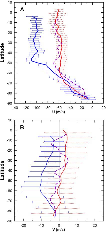
Fig. 6.22 Averaged zonal (top) and meridional (bottom) wind profiles in Venus’s southern hemisphere at cloud level (April 2006-June 2007), as a function of latitude. Cloud tracers were measured at three wavelengths probing different altitudes: ultraviolet (380 nm, upper cloud \(\sim 66\) km, day; blue), near-infrared (980 nm, upper cloud \(\sim 61\) km, day; violet), and infrared (1.74 µm, lower cloud \(\sim 47\) km, night; red). Zonal winds at low latitudes reach \(\sim 105\) m s\(^{-1}\) at the cloud tops but only \(\sim 60\)-\(70\) m s\(^{-1}\) at the cloud base; meridional winds are poleward at the cloud tops with peak \(\sim 10\) m s\(^{-1}\). The cloud-top winds are \(\sim 60\) times faster than the planet’s solid-body rotation, a state known as atmospheric super-rotation. Reproduced from [Sánchez-Lavega et al., 2008], Fig. 2.

6.6.3. Jupiter: the Great Red Spot

Jupiter’s Great Red Spot (GRS) is the largest and longest-lived storm in the solar system: an anticyclonic vortex larger than Earth, with winds reaching \(\sim\)120 m s\(^{-1}\) at its periphery, observed continuously since 1830 (Fig. 6.23).

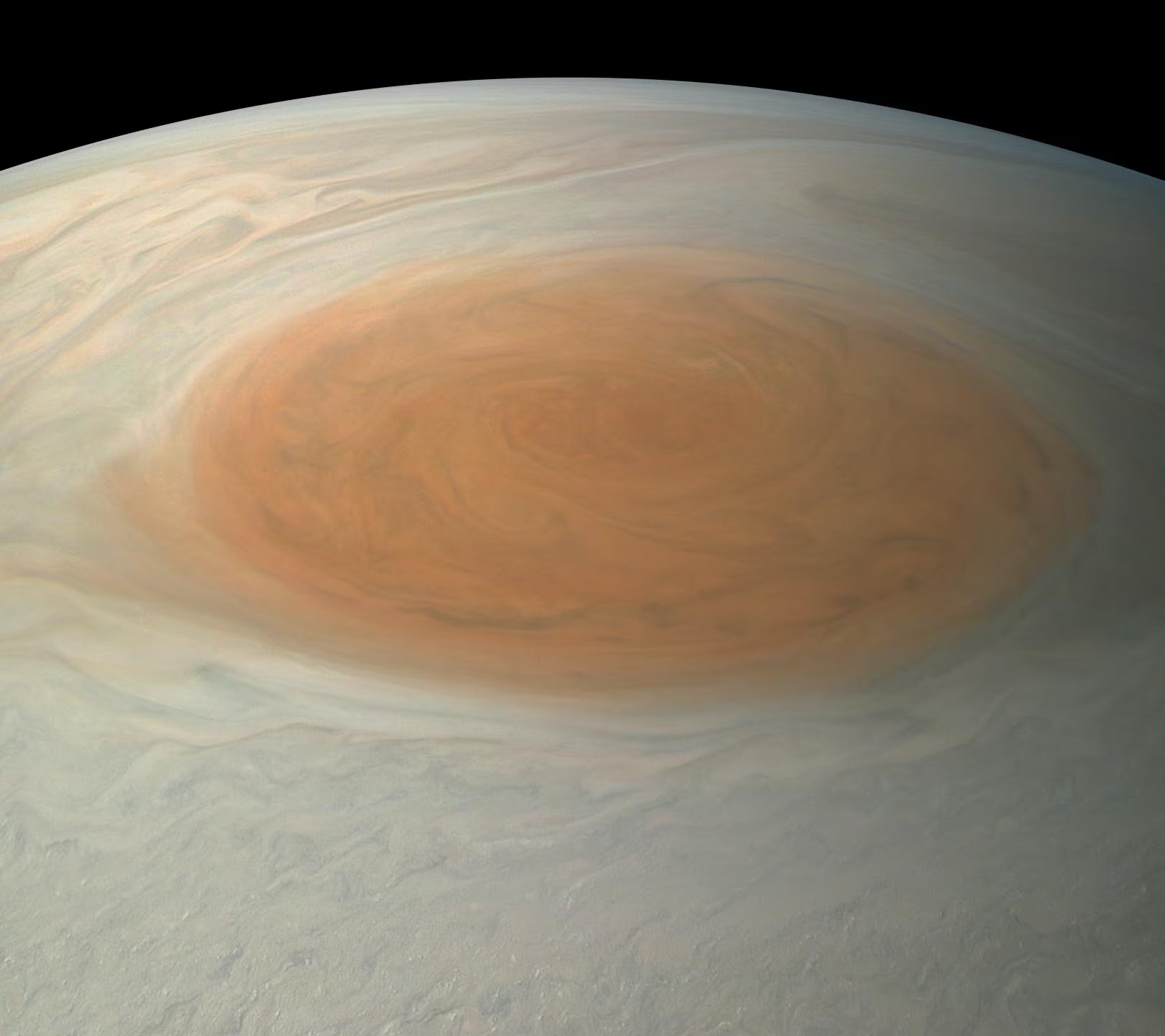
Fig. 6.23 Jupiter’s Great Red Spot and surrounding turbulent atmosphere, imaged by NASA’s Juno spacecraft during a close flyby. The Great Red Spot is an anticyclonic storm larger than Earth that has persisted for centuries. The surrounding vortices and chaotic cloud patterns reveal the intense turbulence of Jupiter’s upper troposphere. Credit: NASA/JPL-Caltech/SwRI/MSSS, public domain.

The GRS is sustained between opposing zonal jets by absorbing smaller vortices and latent heat release [de Pater and Lissauer, 2010], while Juno reveals stable polygonal clusters of circumpolar cyclones at both poles (Fig. 6.24) [Adriani et al., 2018] (Lecture 11).

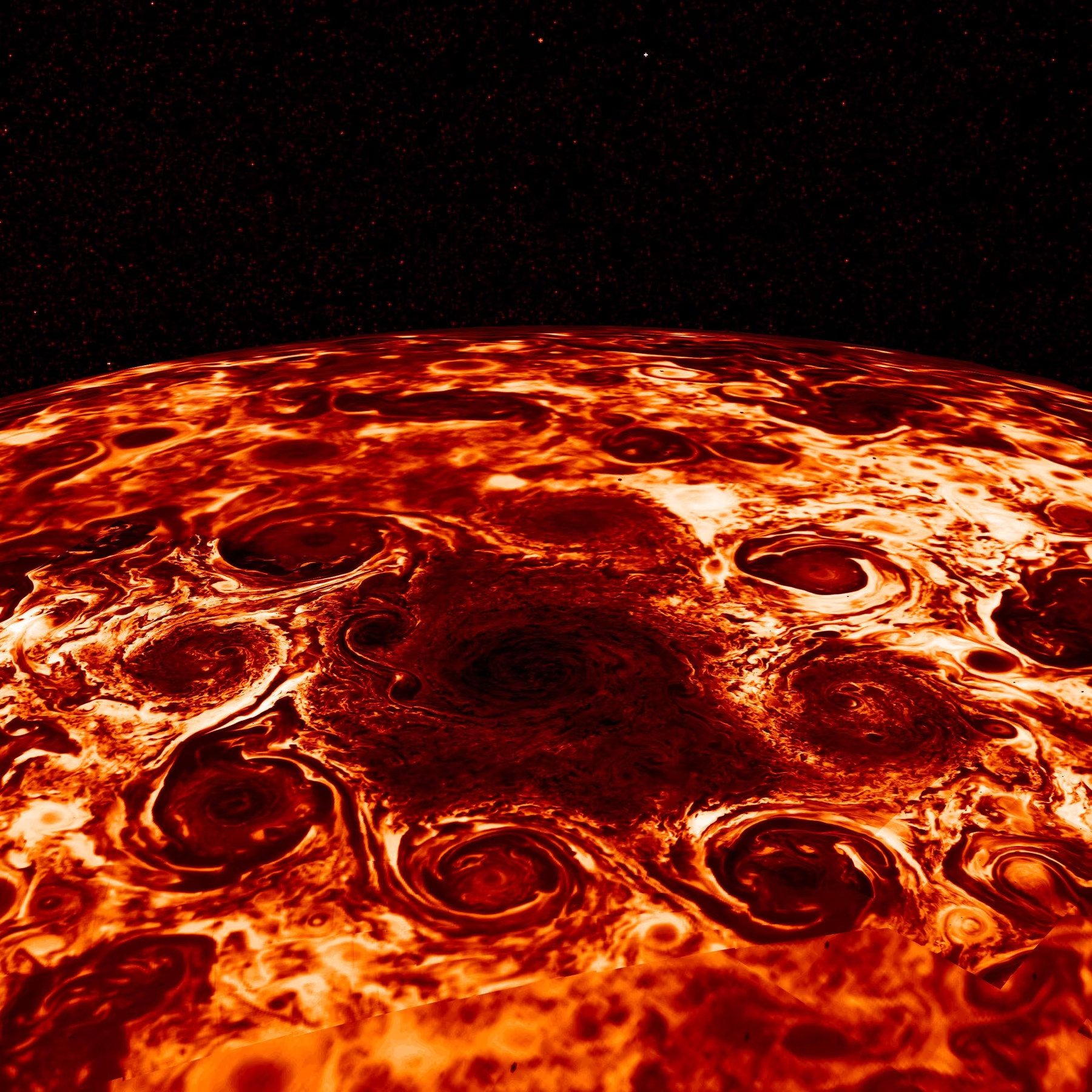
Fig. 6.24 Polar cyclone cluster at Jupiter’s north pole imaged by the JIRAM infrared spectrometer on NASA’s Juno spacecraft. A central cyclone is encircled by eight smaller cyclones in a stable octagonal arrangement, which shows that Jupiter’s atmospheric dynamics produce coherent polygonal vortex patterns analogous to Saturn’s polar hexagonal jet. The cyclones have remained in this configuration over multiple Juno perijoves (the spacecraft’s closest approaches to Jupiter on each orbit) spanning several years, far longer than any Earth analogue. At the south pole, a pentagonal cluster of five circumpolar cyclones remained remarkably stable through perijove 18 (February 2019) [Adriani et al., 2020]; a sixth cyclone briefly joined the southern pentagon in late 2019 but dissipated within about two months without merging, leaving the pentagonal arrangement intact [Mura et al., 2021]. Adapted from Adriani et al. [2018]. Credit: NASA/JPL-Caltech/SwRI/ASI/INAF/JIRAM, public domain.

6.6.4. Saturn: the hexagonal jet stream

Saturn’s north pole hosts one of the most geometrically striking features in the solar system: a persistent hexagonal jet stream (Fig. 6.25) encircling the pole at \(\sim\)78°N latitude, first seen in the Voyager flyby images of 1980-81 and extensively imaged by Cassini.

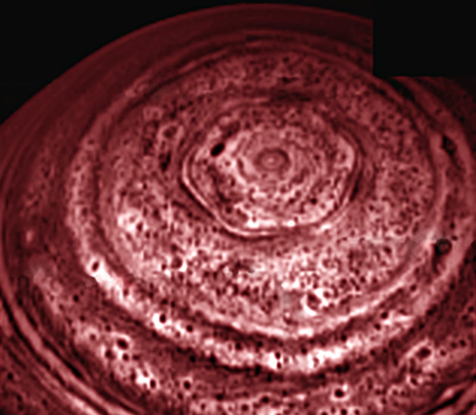
Fig. 6.25 Saturn’s hexagonal jet stream encircling the north pole at \(\sim\)78°N, imaged by NASA’s Cassini spacecraft in November 2012. The hexagonal pattern is interpreted as a stable Rossby wave with six-fold symmetry, sustained by the prograde polar jet at its boundary. The hexagon spans \(\sim\)30,000 km across, larger than Earth’s diameter, and has persisted since its discovery in the Voyager 1 and 2 flyby images of 1980-81. Credit: NASA/JPL-Caltech/SSI/Hampton University, public domain.

The hexagonal shape is explained as a stable Rossby wave, a large-scale atmospheric wave whose restoring force is the variation of the Coriolis parameter with latitude. When the jet stream speed and width satisfy certain resonance conditions, the wave locks into a pattern with a specific number of sides. Laboratory experiments with rotating fluids have reproduced hexagonal and other polygonal patterns under analogous conditions.

Saturn also experiences periodic Great White Storms roughly every 30 years (most recently in 2010), massive convective outbursts that encircle the planet within weeks (Lecture 11).

6.6.5. Neptune: extreme weather on a cold world

Despite receiving only \(\sim\)1/900th of Earth’s solar flux, Neptune sustains the fastest winds in the solar system, with a retrograde equatorial jet reaching \(\sim\)400 m s\(^{-1}\) [Smith et al., 1989], driven by an internal heat excess that also powers transient dark spot storms (Lecture 11). The prominent anticyclonic storm imaged during the Voyager 2 flyby is shown in Fig. 6.26.

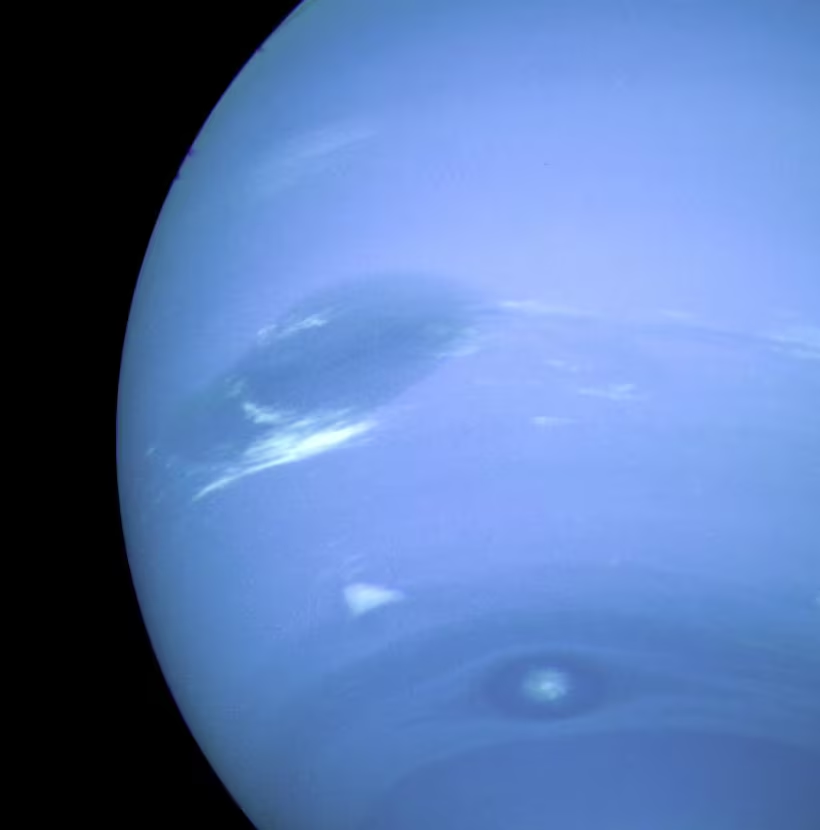
Fig. 6.26 Neptune’s Great Dark Spot (centre-left, with bright “scooter” cloud feature below) and Dark Spot 2 (lower right), imaged by Voyager 2 in August 1989. The Great Dark Spot was a high-pressure anticyclone roughly the size of Earth. The adjacent zonal flow (Neptune’s equatorial retrograde jet reaches \(\sim 400\) m s\(^{-1}\), the fastest winds measured in the solar system) helped confine and transport the storm. Hubble follow-up imaging just a few years later showed that the original Great Dark Spot had dissipated and new dark spots had appeared elsewhere on the planet, which shows that Neptune’s storms are far more transient than Jupiter’s GRS. Credit: NASA/JPL-Caltech, public domain.

6.7. Climate evolution and the faint young Sun

On timescales of billions of years, a planet’s climate is not constant: it evolves in response to changes in the host star’s luminosity, the atmospheric composition, and geological processes. The most celebrated example of this long-term evolution is the faint young Sun paradox [Feulner, 2012].

6.7.1. Solar luminosity evolution

The Sun, like all main-sequence stars, has been gradually brightening as hydrogen is converted to helium in the core. The increasing mean molecular weight requires higher core temperatures to maintain pressure support, which increases the nuclear reaction rate and hence the luminosity. A standard solar evolution model gives [Catling and Kasting, 2017, Gough, 1981]:

(6.3)\[ \frac{L(t)}{\Lsun} \approx \left[1 + \frac{2}{5}\left(1 - \frac{t}{t_\odot}\right)\right]^{-1} \]

where \(t\) is the time since the Sun’s formation and \(t_\odot \approx 4.57\) Gyr is the present age of the Sun. At formation (\(t = 0\)):

\[ \frac{L(0)}{\Lsun} = \frac{1}{1.4} \approx 0.71 \]

The early Sun was \(\sim\)30% less luminous than today. Even 4 Gyr ago (when the first evidence for life on Earth appears), the Sun was still \(\sim\)25% fainter (Fig. 6.27).

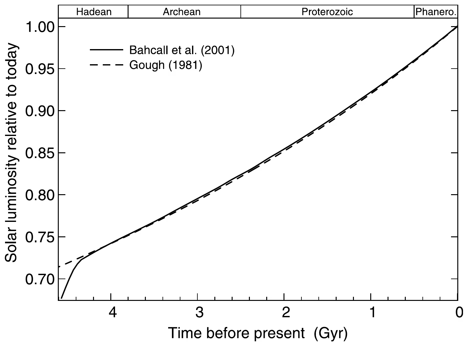
Fig. 6.27 Evolution of solar luminosity over the four geologic eons (Hadean, Archean, Proterozoic, Phanerozoic; labelled bands at top), normalised to the present-day value. The standard-solar-model curve from Bahcall et al. (2001) (solid line) and the analytic approximation by Gough [1981] (dashed line, Eq. (6.3)) agree closely over the past 4 Gyr. At \(t = 0\) (left edge, \(\sim 4.5\) Gyr ago) the Sun was about \(30\%\) less luminous than today; the Archean climate problem of maintaining liquid surface water under this faint young Sun is the faint young Sun paradox. Reproduced from [Feulner, 2012], Fig. 1.

6.7.2. The paradox

A 30% reduction in solar luminosity would reduce Earth’s equilibrium temperature from 255 K to:

\[ T_{\mathrm{eq}} = 255 \times (0.71)^{1/4} \approx 234 \text{ K} \]

Combined with a greenhouse effect similar to today’s, this would yield a surface temperature well below freezing: the entire ocean should have been frozen solid. Yet geological evidence tells a strikingly different story:

• Zircon crystals from 4.4 Ga show oxygen isotope ratios (\(\delta^{18}\mathrm{O}\)) consistent with liquid water interacting with rock at the surface.

• Pillow basalts (lava cooled underwater) and sedimentary rocks (requiring liquid water for transport and deposition) date back to at least 3.8 Ga.

• Stromatolites (microbial mat fossils) at 3.5 Ga and possible carbon isotope signatures of life at 3.8 Ga imply liquid water and conditions warm enough for biology.

This contradiction, a faint Sun that should have frozen the Earth versus geological evidence for liquid water, is the faint young Sun paradox, first articulated by Sagan and Mullen [1972].

Fig. 6.28 shows the temperature gap and the evidence that contradicts it.

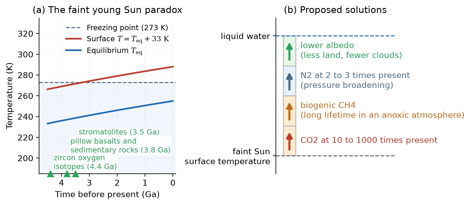
Fig. 6.28 (a) The faint young Sun paradox: the equilibrium temperature \(T_\mathrm{eq} = 255\,(L/L_\odot)^{1/4}\) K for a solar luminosity that rises linearly from 0.70 of today’s value at 4.5 Ga (an approximation to the solar evolution), the surface temperature with today’s greenhouse warming of 33 K added, and the freezing point at 273 K. In this approximation the surface stays below freezing until about 3.2 Ga, yet zircon oxygen isotopes (4.4 Ga), pillow basalts and sedimentary rocks (3.8 Ga) and stromatolites (3.5 Ga) record liquid water. (b) The proposed warming contributions stacked without numerical values: CO\(_2\) at 10 to 1000 times present, biogenic CH\(_4\), N\(_2\) at 2 to 3 times present, and a lower albedo. Course-original figure.

6.7.3. Possible solutions

Several mechanisms have been proposed to resolve the paradox [Feulner, 2012]:

• Enhanced \(\mathrm{CO_2}\) greenhouse: If the early atmosphere contained 10–1000 times more \(\mathrm{CO_2}\) than today (plausible: with less continental area exposed to weathering on the early Earth, the carbonate-silicate thermostat of the next section settles at a higher \(\mathrm{CO_2}\) level), the enhanced greenhouse warming could compensate for the weaker Sun.

• Methane greenhouse: Biogenic \(\mathrm{CH_4}\) from early methanogens could have provided additional greenhouse warming. \(\mathrm{CH_4}\) is a potent greenhouse gas, and in an anoxic (oxygen-free) early atmosphere, it would have had a much longer lifetime than today.

• \(\mathrm{N_2}\) pressure broadening: A thicker \(\mathrm{N_2}\) atmosphere (2–3 times present levels) would enhance greenhouse warming through pressure broadening of \(\mathrm{CO_2}\) and \(\mathrm{H_2O}\) absorption lines.

• Lower albedo: Without continents (less land area in the Archean) and potentially fewer clouds, the early Earth may have reflected less sunlight, absorbing more energy despite the lower luminosity.

The most likely resolution is a combination of elevated \(\mathrm{CO_2}\) and \(\mathrm{CH_4}\) concentrations, regulated by the carbonate-silicate cycle (next section).

Panel (b) of Fig. 6.28 stacks these four contributions.

6.7.4. The Mars climate puzzle

Despite receiving less than half of Earth’s solar flux, early Mars shows compelling geological evidence for warm, wet conditions during the Noachian period (\(>3.7\) Ga) with valley networks carved by flowing water (Fig. 6.29) [Wordsworth, 2016] (Lecture 10).

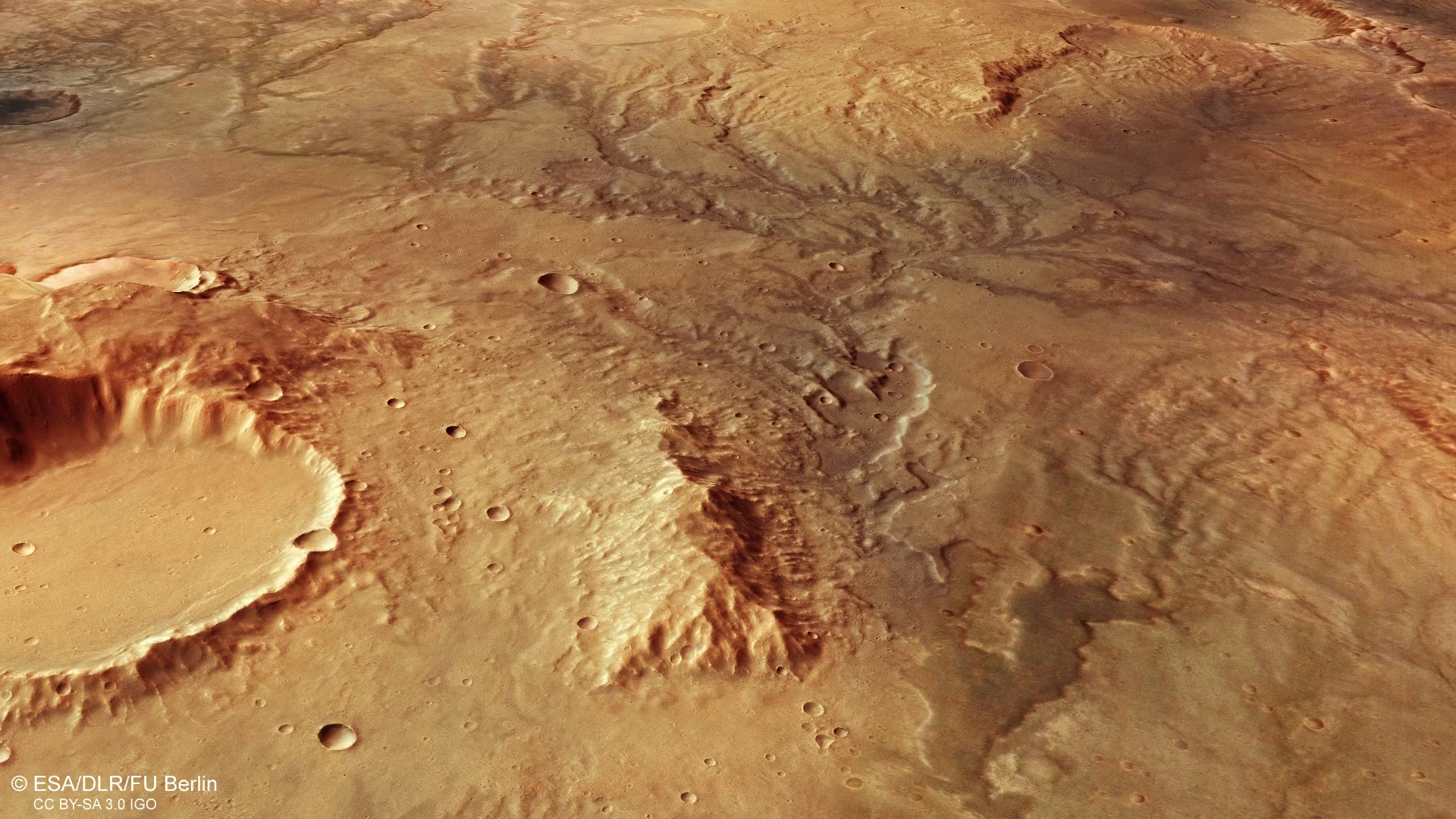
Fig. 6.29 Perspective view of an ancient valley network in the Noachian highlands of Mars, derived from the Mars Express High Resolution Stereo Camera (HRSC) digital terrain model. The dendritic, river-like channel pattern requires sustained surface runoff and is incompatible with the present-day Mars climate, where mean surface temperature is \(\sim\)215 K and surface pressure is below the triple point of water. Such networks are among the strongest geological constraints on the warm-wet Noachian climate problem discussed by Wordsworth [2016]. Credit: ESA / DLR / FU Berlin (G. Neukum), CC BY-SA 3.0 IGO.

6.7.5. Orbital forcing: Milankovitch cycles

Stellar luminosity sets the trend over billions of years. On timescales of tens of thousands of years the dominant forcing is instead geometric: the orbit and the spin axis of the planet both change slowly, driven by the gravitational pull of the other planets. Three quantities matter, and together they are known as the Milankovitch cycles (Fig. 6.30).

• Obliquity \(\varepsilon\), the tilt of the spin axis away from the orbit normal, oscillates between \(22.1^\circ\) and \(24.5^\circ\) with a period near 41 kyr. A larger tilt strengthens the seasonal contrast at both poles at once.

• Eccentricity \(e\), the departure of the orbit from a circle, varies between \(e \approx 0\) and \(e \approx 0.06\) with beating periods near 100 and 400 kyr. It controls how much the star-planet distance changes over one orbit.

• Climatic precession, the wobble of the spin axis combined with the slow turning of the orbital ellipse itself, has a period of 19-23 kyr. It sets which season falls at perihelion, and its amplitude is scaled by \(e\), so the two are not independent. The combination \(e \sin \varpi\), where \(\varpi\) is the longitude of perihelion, is the quantity that enters the insolation.

The essential point is that obliquity and precession move sunlight around; they do not add any. Averaged over a full orbit and over the whole globe, the flux a planet receives is \(L_\star / (4 \pi a^2 \sqrt{1 - e^2})\), which is independent of both the tilt and the phase of the wobble. Only eccentricity enters, and weakly: swinging \(e\) from 0 to 0.06 changes the annual global mean by less than 0.2%. What the cycles do change, by tens of watts per square metre, is the insolation at a given latitude in a given season. Summer insolation at \(65^\circ\)N is the classical index, because that is where the northern ice sheets grow and melt, and a cool summer that fails to melt the previous winter’s snow is what lets an ice sheet survive.

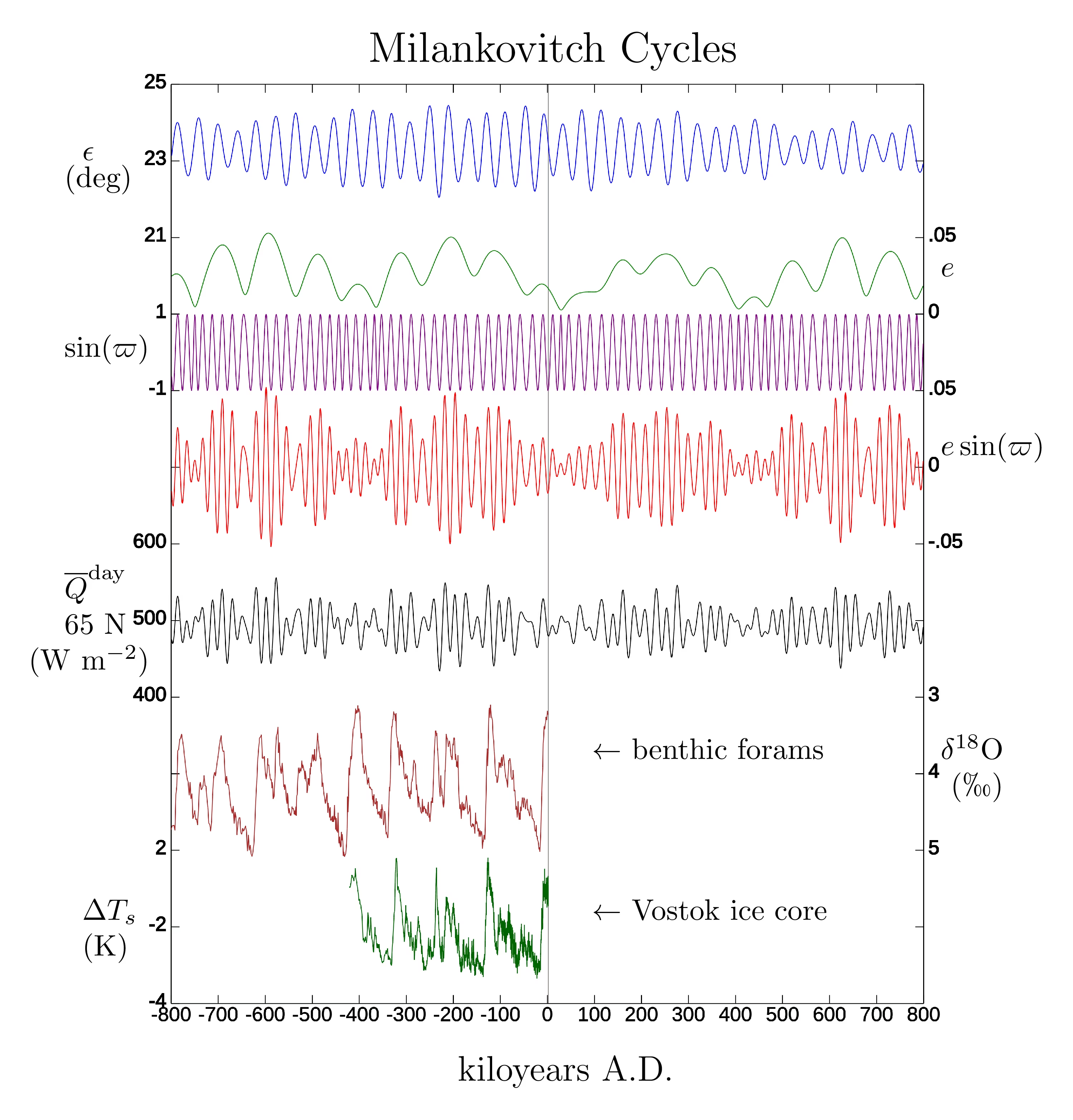
Fig. 6.30 The Milankovitch cycles over the past and next 800 kyr. From top: obliquity \(\varepsilon\); eccentricity \(e\); the precession term \(\sin \varpi\) and the precession index \(e \sin \varpi\); the resulting daily-mean summer insolation at \(65^\circ\)N; and two climate records, the \(\delta^{18}\mathrm{O}\) of benthic foraminifera and the temperature anomaly from the Vostok ice core. The orbital quantities are computed, not measured; the two lowest curves are data. The 100 kyr rhythm of the glacial cycles in the lower panels has no counterpart of matching strength in the insolation curve above it, which is the unsolved part of the problem. Credit: Wikimedia Commons, CC BY-SA.

Spectral analysis of ocean sediment cores confirms that these orbital frequencies pace the ice ages [Hays et al., 1976]; the orbital solution itself is computed reliably over the last 40 Myr [Laskar et al., 2004], and non-linear climate feedbacks are required to explain the dominant 100 kyr rhythm.

6.7.6. Climate feedbacks

The stability of a planet’s climate depends on feedback mechanisms, processes where a change in temperature triggers secondary effects that either amplify (positive feedback) or counteract (negative feedback) the original change:

• Ice-albedo feedback (positive): If the planet cools, ice and snow expand \(\Rightarrow\) the surface becomes more reflective (higher albedo) \(\Rightarrow\) less sunlight is absorbed \(\Rightarrow\) further cooling. Pushed far enough, this feedback can lock a planet into a globally frozen snowball state, as may have happened on Earth during the Neoproterozoic. The energy balance behind this behaviour is set out below.

• Water vapour feedback (positive): Warming increases atmospheric water vapour, amplifying the greenhouse effect [IPCC, 2021], which in the extreme limit triggers a runaway greenhouse (Lecture 9).

• Cloud feedback (complex): Low-altitude clouds reflect sunlight (cooling), while high-altitude cirrus clouds trap infrared radiation (warming). The net cloud feedback is the largest source of uncertainty in Earth climate models and is one of the key unknowns for exoplanet climate predictions (Lecture 13).

6.7.6.1. Snowball Earth and climate bistability

The ice-albedo feedback is the clearest case of how a single feedback can give a planet more than one stable climate. Taken to its extreme it produces a snowball Earth (Fig. 6.31), a state in which ice and snow cover almost the whole surface, from the poles to the equator. The evidence is geological: glacial deposits laid down at tropical latitudes show that Earth entered such states around 717 and 635 Ma [Hoffman et al., 2017, Hoffman et al., 1998].

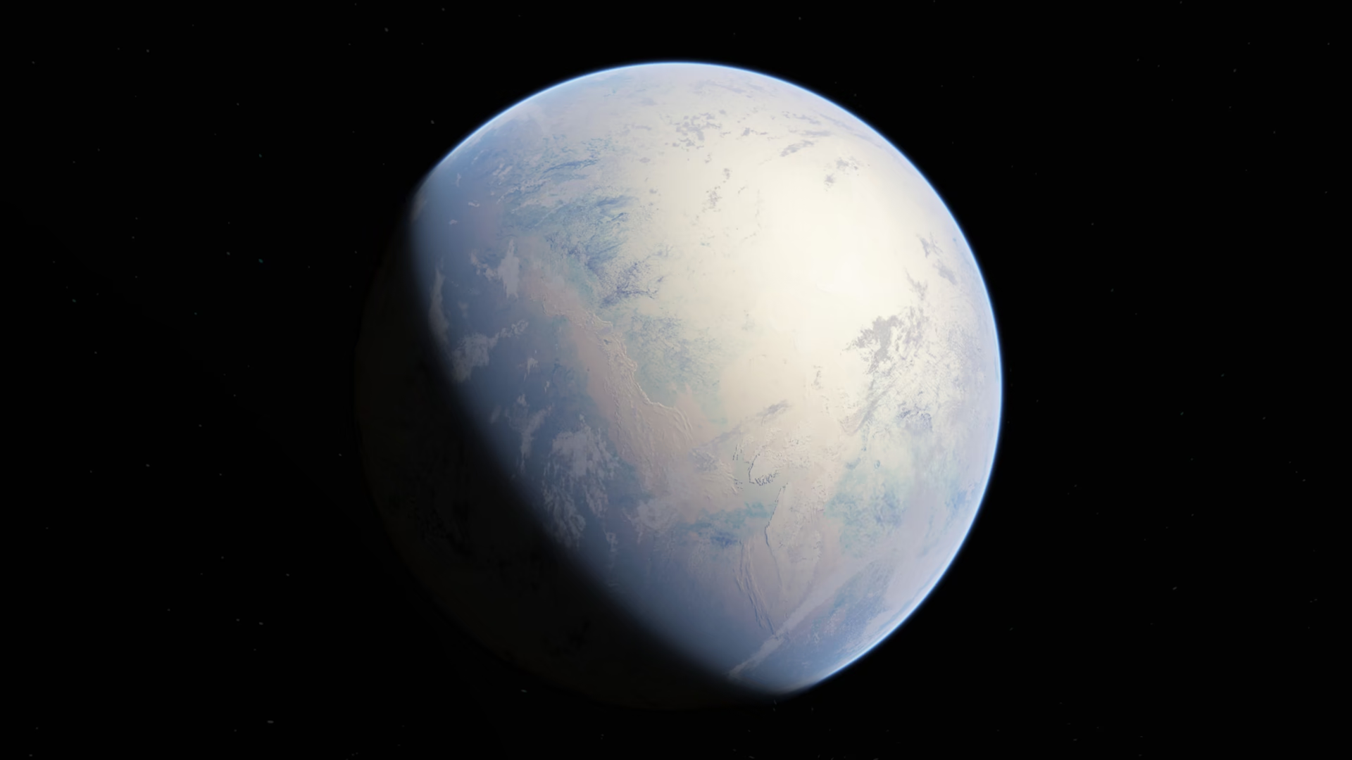
Fig. 6.31 Artist’s impression of a fully ice-covered “snowball” Earth, with the continents buried under ice and only faint outlines showing through. A bright frozen surface reflects most of the incoming sunlight, which is what makes the snowball state so stable. Credit: Oleg Kuznetsov (3depix.com), CC BY-SA 4.0.

A planet’s surface temperature settles where the sunlight it absorbs equals the thermal radiation it emits to space. Fig. 6.32 plots both terms against surface temperature \(T\), and the two behave very differently. The emitted radiation (red) follows the grey-body law \(\varepsilon \sigma T^4\) and rises smoothly and steeply with temperature, because a warmer surface always radiates more. The absorbed sunlight (blue) is \((1 - \alpha(T))\,S/4\), where \(S\) is the stellar flux and \(\alpha(T)\) the planetary albedo, so its temperature dependence enters only through the albedo. That albedo is not fixed: a frozen surface is bright (\(\alpha \approx 0.6\)), an ice-free surface dark (\(\alpha \approx 0.3\)). As the planet warms through the freezing range and its ice retreats, the albedo falls, so the blue curve climbs steeply across a narrow band of temperature and is nearly flat on either side of it.

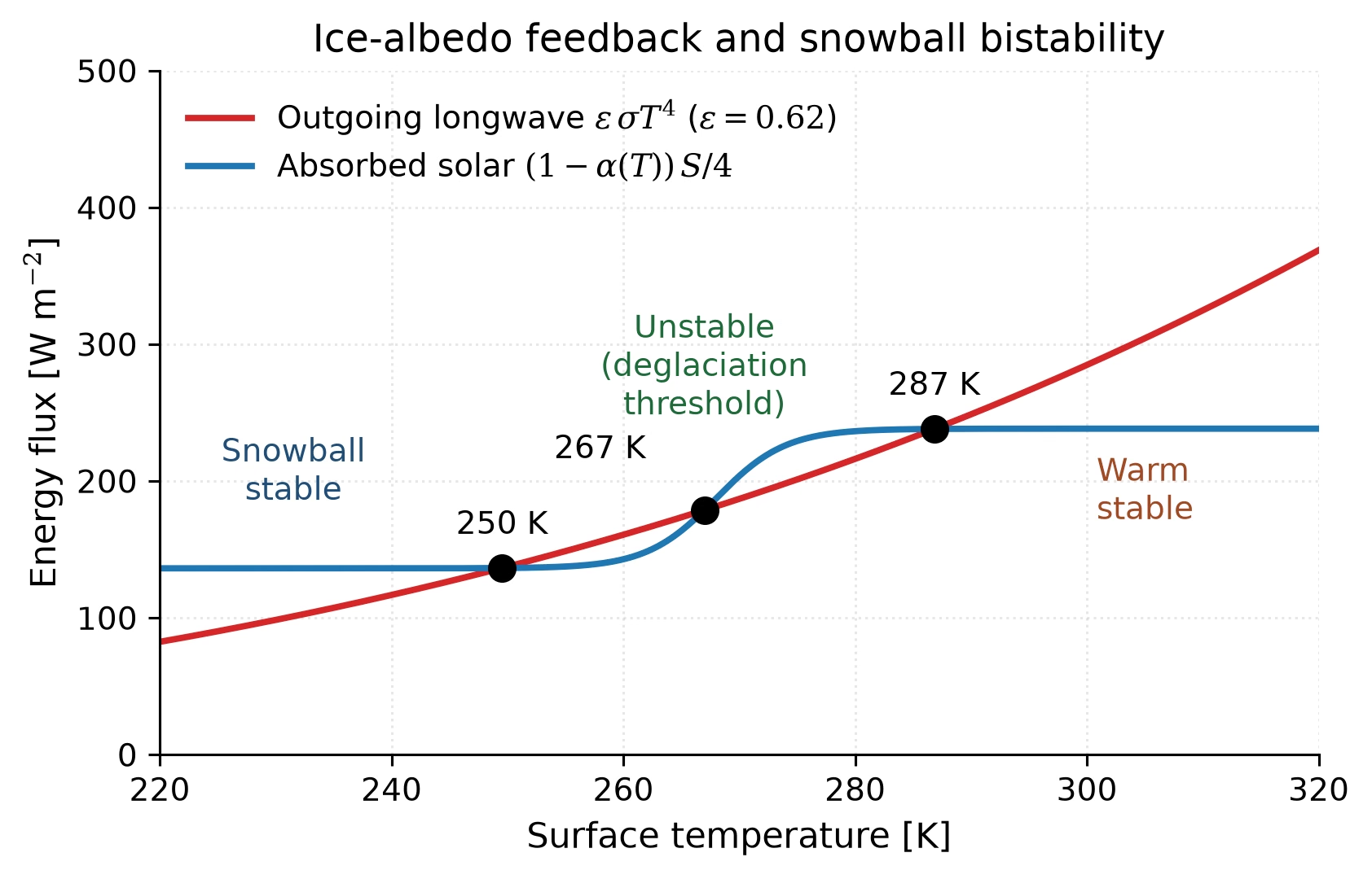
Fig. 6.32 Energy-balance illustration of the ice-albedo feedback and snowball bistability. The red curve is the outgoing longwave radiation \(\varepsilon \sigma T^4\) with a fixed grey emissivity \(\varepsilon = 0.62\) (a constant greenhouse), and the blue curve is the absorbed solar flux \((1 - \alpha(T))\,S/4\) with a temperature-dependent albedo that drops from \(\sim\)0.6 (ice-covered) to \(\sim\)0.3 (ice-free) across the freezing region. Three energy-balance equilibria exist: a stable cold snowball state (left intersection), an unstable deglaciation threshold (middle), and a stable warm state (right). Pushing the system across the unstable middle point triggers a runaway transition. The snowball events of the Neoproterozoic (\(\sim\)717 and \(\sim\)635 Ma) are interpreted as global excursions of this bifurcation diagram [Hoffman et al., 2017, Hoffman et al., 1998]. Course-original figure.

Wherever the two curves cross, absorbed and emitted power balance, so each crossing is an equilibrium. For the values shown they cross three times. Their stability follows from a simple slope test. At the cold (\(\sim\)250 K) and warm (\(\sim\)287 K) crossings the radiation curve is the steeper of the two, so a small warming radiates away more energy than it gains and the planet slides back to the crossing; a small cooling is undone the same way. Both are stable climates. The middle crossing (\(\sim\)267 K) is different: there the absorbed-sunlight curve is steeper, so a small warming absorbs more than it emits and the planet keeps warming, while a small cooling runs away downward. This state is an unstable deglaciation threshold, and no planet can rest on it.

Two stable climates for the same stellar flux is a bistability. Which one a planet occupies then depends on its history, not on the sunlight alone. Cool a warm world past the middle threshold, by a fall in greenhouse gases or in stellar flux, and it drops onto the snowball branch; climbing back out means crossing the threshold again from the cold side. Escape is hard. The bright frozen surface reflects most of the incoming sunlight, so only a large greenhouse forcing can lift the blue curve far enough to erase the cold crossing. On Earth that forcing builds up as volcanic \(\mathrm{CO_2}\) accumulates in an atmosphere where the ice cover has shut down the silicate weathering that normally removes it, the negative feedback described in the next section.

6.8. The carbonate-silicate cycle

Earth has maintained liquid water at its surface for at least 4.4 billion years despite a 30% increase in solar luminosity. This remarkable stability requires a powerful negative feedback mechanism: the carbonate-silicate cycle, first described by [Walker et al., 1981].

6.8.1. The Urey reaction

The cycle is built on the chemical weathering of silicate rocks by atmospheric \(\mathrm{CO_2}\) dissolved in rainwater. The net reaction, with water as the medium that dissolves the \(\mathrm{CO_2}\) and carries the ions, is:

\[ \mathrm{CaSiO_3} + \mathrm{CO_2} \longrightarrow \mathrm{CaCO_3} + \mathrm{SiO_2} \]

This is sometimes called the Urey reaction. In words: carbon dioxide from the atmosphere dissolves in rainwater to form a weak acid, which reacts with silicate minerals in surface rocks. The products (calcium carbonate, \(\mathrm{CaCO_3}\), limestone; and silica, \(\mathrm{SiO_2}\)) are transported by rivers to the ocean, where the carbonate precipitates, that is, comes out of solution as solid grains (biologically, as the shells and skeletons of marine organisms, or abiotically), and is deposited on the ocean floor as sedimentary rock.

The net effect is to draw \(\mathrm{CO_2}\) out of the atmosphere and lock it into carbonate rocks. This is the long-term carbon sink.

Fig. 6.33 follows the carbon along this pathway.

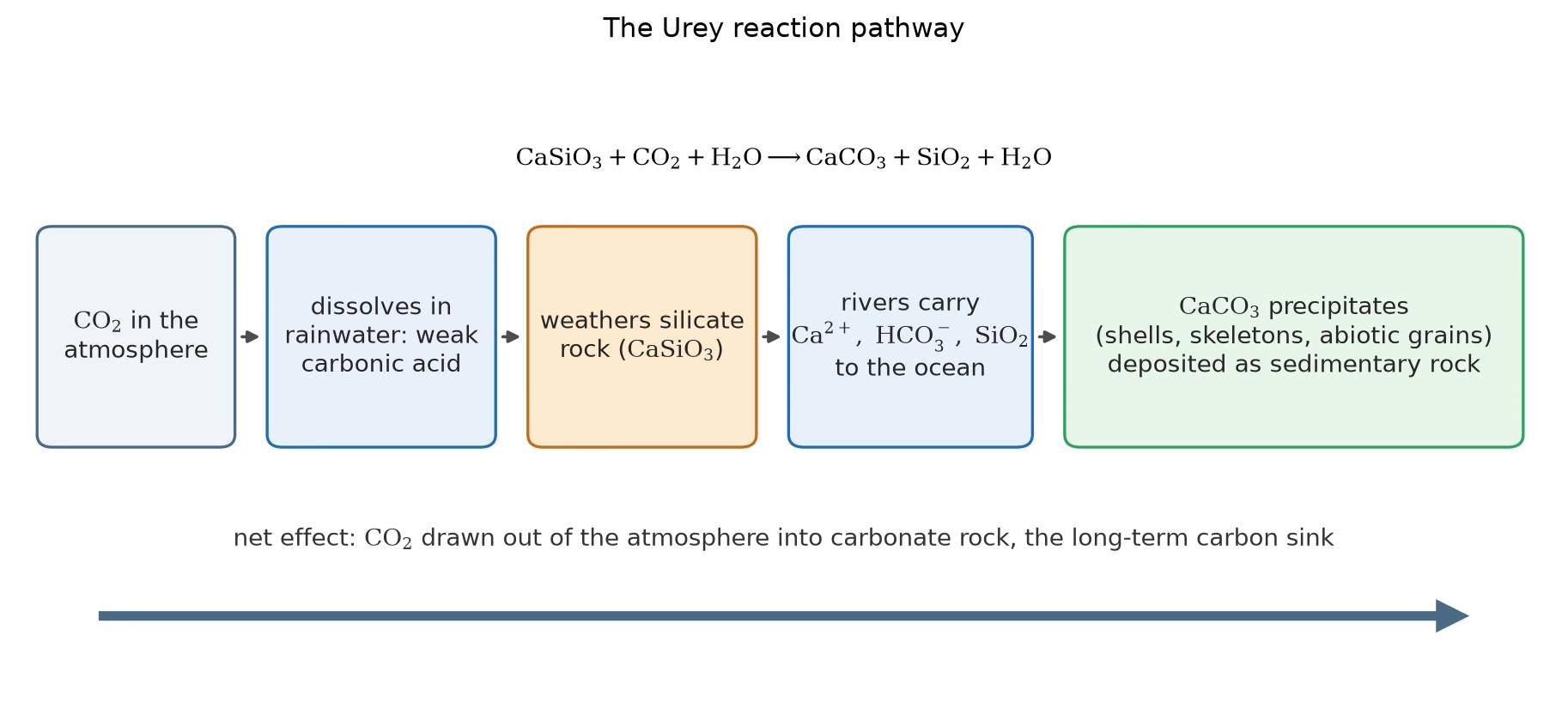
Fig. 6.33 The Urey reaction pathway: atmospheric CO\(_2\) dissolves in rainwater as a weak carbonic acid, weathers silicate rock (CaSiO\(_3\)), and rivers carry the dissolved calcium, bicarbonate and silica to the ocean, where CaCO\(_3\) precipitates as shells, skeletons or abiotic grains and is deposited as sedimentary rock. The net reaction CaSiO\(_3\) + CO\(_2\) \(\rightarrow\) CaCO\(_3\) + SiO\(_2\), with water as the medium, draws CO\(_2\) out of the atmosphere into carbonate rock, the long-term carbon sink. Course-original figure.

6.8.2. Volcanic outgassing: the carbon source

The cycle is closed by plate tectonics. Carbonate-bearing ocean floor is subducted into the mantle, where high temperatures and pressures decompose the carbonates, releasing \(\mathrm{CO_2}\). This \(\mathrm{CO_2}\) is returned to the atmosphere through volcanic outgassing, the long-term carbon source.

6.8.3. The negative feedback

The weathering rate depends strongly on temperature through an Arrhenius-type dependence: chemical reactions proceed faster at higher temperatures. Additionally, a warmer climate produces more rainfall (more water evaporates from the oceans), which further accelerates weathering. This creates a powerful negative feedback loop [Walker et al., 1981]:

1. If the planet warms (e.g., due to increasing solar luminosity or volcanic outgassing): more rainfall + faster chemical reactions → weathering rate increases → more \(\mathrm{CO_2}\) is drawn out of the atmosphere → greenhouse weakens → planet cools back down.

2. If the planet cools (e.g., due to reduced volcanic activity or orbital changes): less rainfall + slower reactions → weathering rate decreases → \(\mathrm{CO_2}\) from volcanism accumulates in the atmosphere → greenhouse strengthens → planet warms back up.

Both loops are usually captured in climate models by a single parameterisation of the weathering rate \(W\) as a function of surface temperature \(T\),

(6.4)\[ W(T) = W_0 \exp\!\left( \frac{T - T_0}{T_e} \right), \]

where \(W_0\) is the weathering rate at a reference temperature \(T_0\) and \(T_e\) is an \(e\)-folding temperature. For Earth \(T_e \approx 10\) K, a value that absorbs both the Arrhenius kinetics of the mineral reactions and the increase in runoff with temperature. Two consequences follow directly. Doubling the weathering rate requires a warming of \(T_e \ln 2 \approx 7\) K, and halving it requires a cooling of the same amount; the feedback is therefore strong enough to matter but gentle enough that the planet is not driven to an extreme by a small perturbation. And in steady state the sink must match the source, \(W = V\), where \(V\) is the volcanic outgassing rate. It is that balance, not the total carbon inventory, which fixes the atmospheric \(p\mathrm{CO_2}\) of a planet: raise the volcanic supply and the atmosphere warms only until weathering has sped up enough to remove the extra carbon again.

This thermostat operates on geological timescales of \(\sim 10^5\)–\(10^6\) yr, long by human standards but short compared to geological time. It is the primary reason Earth has maintained habitable surface temperatures for over 4 billion years despite the 30% increase in solar luminosity. The geologic cycle as a whole is summarised in Fig. 6.35; the modern plate-tectonic version of the loop is reviewed by Foley [2024] and drawn in Fig. 6.34.

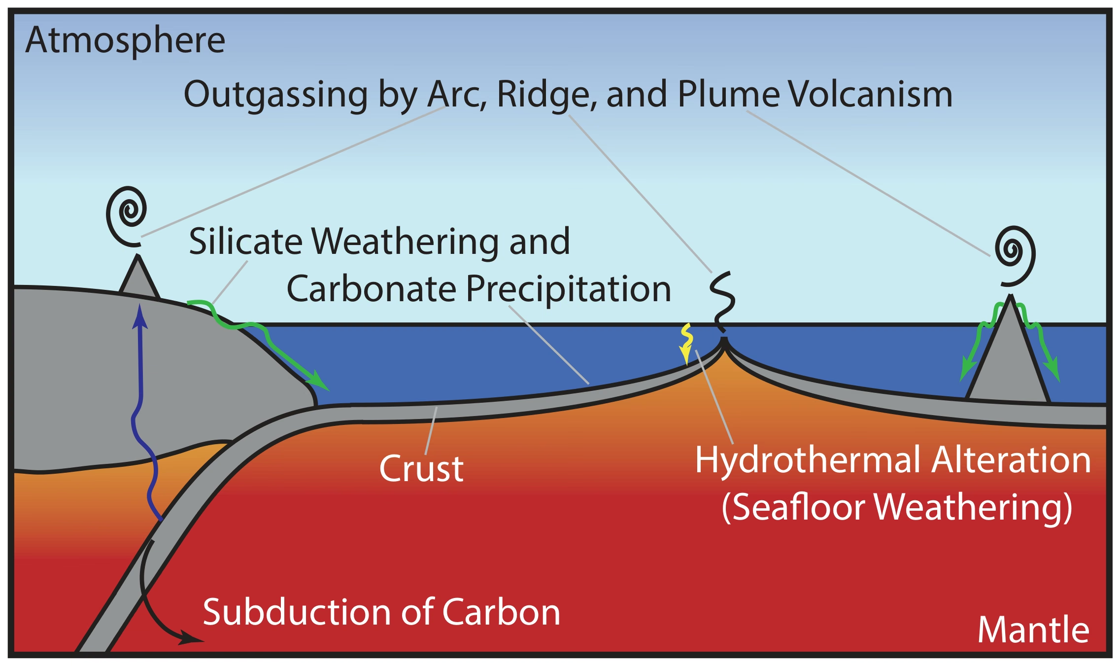
Fig. 6.34 Schematic diagram of the carbonate-silicate cycle as it operates on the modern-day, plate-tectonic Earth. \(\mathrm{CO_2}\) released from the mantle by arc, ridge, and plume volcanism enters the atmosphere; silicate weathering and carbonate precipitation transfer carbon from the atmosphere to the crust; hydrothermal alteration of seafloor basalts (seafloor weathering) is a secondary sink; subduction returns carbon to the mantle. Negative feedback: higher temperature accelerates weathering, drains atmospheric \(\mathrm{CO_2}\), cools the climate. The loop fails on Venus, which lost its liquid water, and on Mars, whose volcanic return path shut down as the interior cooled, as discussed below. Reproduced from [Foley, 2024], Fig. 6.

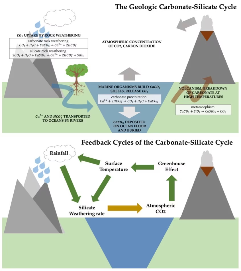
Fig. 6.35 The carbonate-silicate cycle, Earth’s long-term climate thermostat. Top: The geologic cycle: atmospheric \(\mathrm{CO_2}\) dissolves in rainwater and weathers silicate rocks, producing carbonates that are transported to the ocean and deposited as sediments. Subduction and volcanism return the \(\mathrm{CO_2}\) to the atmosphere, closing the cycle. Bottom: The feedback loops: surface temperature, rainfall, silicate weathering rate, atmospheric \(\mathrm{CO_2}\), and the greenhouse effect are linked in a negative feedback that stabilises the climate over geological timescales. Credit: Wikimedia Commons, CC BY-SA 4.0.

6.8.4. Venus and Mars: failed thermostats

The carbonate-silicate cycle requires two essential ingredients: liquid water (to dissolve \(\mathrm{CO_2}\) and weather rocks) and active volcanism (to recycle carbon). Without either, the thermostat fails:

• Venus: Once Venus lost its surface water, likely through the runaway greenhouse and hydrogen escape to space, silicate weathering ceased and volcanic \(\mathrm{CO_2}\) accumulated to the present 92 bar without a carbon sink (Lecture 9).

• Mars: As its interior cooled and volcanism largely ceased by the end of the Hesperian (\(\sim\)3 Ga), the volcanic \(\mathrm{CO_2}\) source broke while silicate weathering drew \(\mathrm{CO_2}\) down into carbonates and the rest was probably lost to space, leaving the modern 6 mbar atmosphere (Lecture 10).

The requirement for both liquid water and active volcanism to maintain the carbonate-silicate cycle has profound implications for planetary habitability: a planet needs both the right temperature and the right geological activity to sustain that temperature over billions of years. This theme will return in Lecture 14 when we discuss the habitability of exoplanets.

Fig. 6.36 sorts the three planets by the two ingredients.

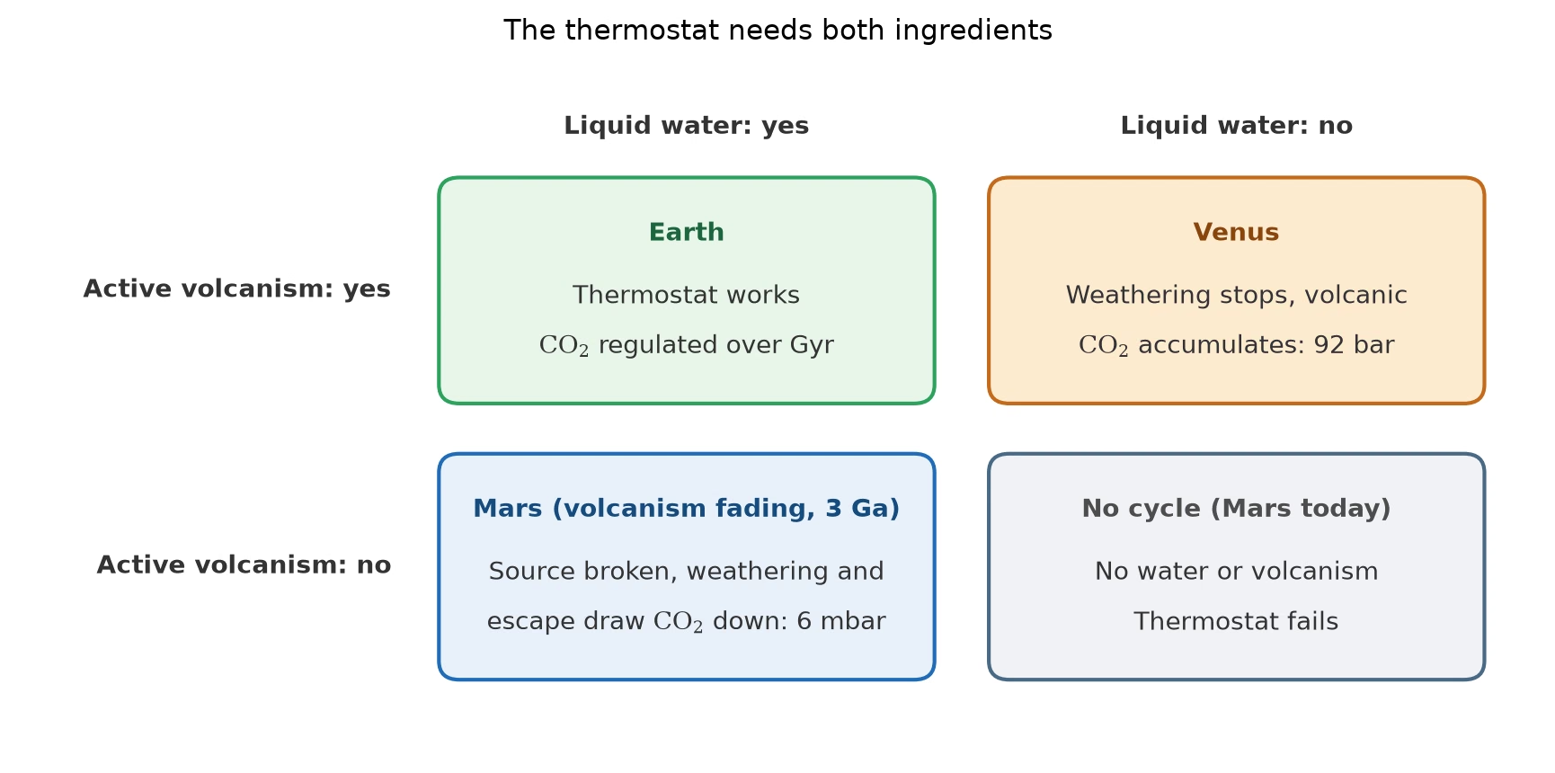
Fig. 6.36 The carbonate-silicate thermostat needs both liquid water and active volcanism. Earth has both and regulates CO\(_2\) over billions of years; Venus lost its water, so weathering stopped and volcanic CO\(_2\) accumulated to 92 bar; on Mars the volcanic source faded after about 3 Ga while weathering and escape to space drew CO\(_2\) down to the present 6 mbar, and today Mars has neither liquid water nor active volcanism, so no cycle runs. Course-original figure.

6.9. Recent advances

In 2020, a team reported a tentative detection of phosphine (\(\mathrm{PH_3}\)) in the cloud decks of Venus using millimetre-wavelength spectroscopy [Greaves et al., 2021], sparking intense debate about possible biological or unknown chemical sources. Independent reanalyses contested the detection, showing among other things that mesospheric \(\mathrm{SO_2}\) can reproduce the observed spectral feature, and it remains controversial [Lincowski et al., 2021]; Lecture 14 returns to it as a biosignature case study. Regardless of the outcome, the episode highlighted how little we understand about Venus’s atmospheric chemistry and motivated renewed interest in Venus exploration. ESA’s EnVision orbiter and NASA’s DAVINCI probe (both selected for launch in the early 2030s) will provide new measurements of Venus’s atmospheric composition and surface-atmosphere interactions.

6.10. Looking ahead to Lecture 7

The last three lectures treated planets from the top down: energy budgets, vertical structure, and now clouds, winds, and climate. Lecture 7 moves to the solid surfaces these atmospheres act upon. Impact cratering provides the clocks by which planetary surfaces are dated, volcanism and tectonics resurface them from within, and erosion and weathering, driven by the winds, rain, and chemistry of this lecture, rework them from above. The climate history written into Mars’s valley networks returns there as a geological record to be read.

6.11. References

[Adriani2020]

Adriani, A., Bracco, A., Grassi, D., Moriconi, M. L., Mura, A., Orton, G., Altieri, F., Ingersoll, A., Atreya, S. K., Lunine, J. I., Migliorini, A., and Noschese, R. 2020. “Two-year observations of the Jupiter polar regions by JIRAM on board Juno.” Journal of Geophysical Research: Planets, 125(6):e2019JE006098. doi:10.1029/2019JE006098, https://ui.adsabs.harvard.edu/abs/2020JGRE..12506098A/abstract.

[Adriani2018] (1,2)

Adriani, A., Mura, A., Orton, G., Hansen, C., Altieri, F., Moriconi, M. L., Rogers, J., Eichstädt, G., Momary, T., Ingersoll, A. P., Filacchione, G., Sindoni, G., Tabataba-Vakili, F., Dinelli, B. M., Fabiano, F., Bolton, S. J., Connerney, J. E. P., Atreya, S. K., Lunine, J. I., Tosi, F., Migliorini, A., Grassi, D., Piccioni, G., Noschese, R., Cicchetti, A., Plainaki, C., Olivieri, A., O'Neill, M. E., Turrini, D., Stefani, S., Sordini, R., and Amoroso, M. 2018. “Clusters of cyclones encircling Jupiter's poles.” Nature, 555:216–219. doi:10.1038/nature25491, https://ui.adsabs.harvard.edu/abs/2018Natur.555..216A/abstract.

[Catling2017] (1,2,3,4,5,6,7)

Catling, David C. and Kasting, James F. 2017. Atmospheric Evolution on Inhabited and Lifeless Worlds. Cambridge University Press, Cambridge. doi:10.1017/9781139020558.

[dePaterLissauer2010] (1,2,3,4,5)

de Pater, Imke and Lissauer, Jack J. 2010. Planetary Sciences. Cambridge University Press, Cambridge, 2nd edition. doi:10.1017/cbo9780511780561.

[Feulner2012] (1,2,3)

Feulner, Georg. 2012. “The faint young Sun problem.” Reviews of Geophysics, 50(2):RG2006. doi:10.1029/2011RG000375, https://ui.adsabs.harvard.edu/abs/2012RvGeo..50.2006F/abstract.

[Foley2024] (1,2)

Foley, Bradford J. 2024. “Exoplanet geology: what can we learn from current and future observations?.” Reviews in Mineralogy and Geochemistry, 90:559–594. doi:10.2138/rmg.2024.90.15, https://ui.adsabs.harvard.edu/abs/2024RvMG...90..559F/abstract.

[GarciaMelendo2001]

García-Melendo, Enrique and Sánchez-Lavega, Agustín. 2001. “A study of the stability of Jovian zonal winds from HST images: 1995-2000.” Icarus, 152(2):316–330. doi:10.1006/icar.2001.6646, https://ui.adsabs.harvard.edu/abs/2001Icar..152..316G/abstract.

[Gough1981] (1,2)

Gough, D. O. 1981. “Solar interior structure and luminosity variations.” Solar Physics, 74(1):21–34. doi:10.1007/BF00151270, https://ui.adsabs.harvard.edu/abs/1981SoPh...74...21G/abstract.

[Greaves2021]

Greaves, Jane S., Richards, Anita M. S., Bains, William, Rimmer, Paul B., Sagawa, Hideo, Clements, David L., Seager, Sara, Petkowski, Janusz J., Sousa-Silva, Clara, Ranjan, Sukrit, Drabek-Maunder, Emily, Fraser, Helen J., Cartwright, Annabel, Mueller-Wodarg, Ingo, Zhan, Zhuchang, Friberg, Per, Coulson, Iain, Lee, E'lisa, and Hoge, Jim. 2021. “Phosphine gas in the cloud decks of venus.” Nature Astronomy, 5:655–664. doi:10.1038/s41550-020-1174-4, https://ui.adsabs.harvard.edu/abs/2021NatAs...5..655G/abstract.

[Hays1976]

Hays, J. D., Imbrie, John, and Shackleton, N. J. 1976. “Variations in the Earth's orbit: pacemaker of the ice ages.” Science, 194(4270):1121–1132. doi:10.1126/science.194.4270.1121, https://ui.adsabs.harvard.edu/abs/1976Sci...194.1121H/abstract.

[Held1980]

Held, Isaac M. and Hou, Arthur Y. 1980. “Nonlinear axially symmetric circulations in a nearly inviscid atmosphere.” Journal of the Atmospheric Sciences, 37(3):515–533. doi:10.1175/1520-0469(1980)037<0515:NASCIA>2.0.CO;2, https://journals.ametsoc.org/view/journals/atsc/37/3/1520-0469_1980_037_0515_nascia_2_0_co_2.xml.

[Hoffman2017] (1,2)

Hoffman, Paul F., Abbot, Dorian S., Ashkenazy, Yosef, Benn, Douglas I., Brocks, Jochen J., Cohen, Phoebe A., Cox, Grant M., Creveling, Jessica R., Donnadieu, Yannick, Erwin, Douglas H., Fairchild, Ian J., Ferreira, David, Goodman, Jason C., Halverson, Galen P., Jansen, Malte F., Le Hir, Guillaume, Love, Gordon D., Macdonald, Francis A., Maloof, Adam C., Partin, Camille A., Ramstein, Gilles, Rose, Brian E. J., Rose, Catherine V., Sadler, Peter M., Tziperman, Eli, Voigt, Aiko, and Warren, Stephen G. 2017. “Snowball Earth climate dynamics and Cryogenian geology–geobiology.” Science Advances, 3(11):e1600983. doi:10.1126/sciadv.1600983, https://ui.adsabs.harvard.edu/abs/2017SciA....3E0983H/abstract.

[Hoffman1998] (1,2)

Hoffman, Paul F., Kaufman, Alan J., Halverson, Galen P., and Schrag, Daniel P. 1998. “A Neoproterozoic snowball Earth.” Science, 281(5381):1342–1346. doi:10.1126/science.281.5381.1342, https://ui.adsabs.harvard.edu/abs/1998Sci...281.1342H/abstract.

[Kaspi2018] (1,2)

Kaspi, Y., Galanti, E., Hubbard, W. B., Stevenson, D. J., Bolton, S. J., Iess, L., Guillot, T., Bloxham, J., Connerney, J. E. P., Cao, H., Durante, D., Folkner, W. M., Helled, R., Ingersoll, A. P., Levin, S. M., Lunine, J. I., Miguel, Y., Militzer, B., Parisi, M., and Wahl, S. M. 2018. “Jupiter's atmospheric jet streams extend thousands of kilometres deep.” Nature, 555:223–226. doi:10.1038/nature25793, https://ui.adsabs.harvard.edu/abs/2018Natur.555..223K/abstract.

[Laskar2004]

Laskar, J., Robutel, P., Joutel, F., Gastineau, M., Correia, A. C. M., and Levrard, B. 2004. “A long-term numerical solution for the insolation quantities of the Earth.” Astronomy & Astrophysics, 428(1):261–285. doi:10.1051/0004-6361:20041335, https://ui.adsabs.harvard.edu/abs/2004A&A...428..261L/abstract.

[Lincowski2021]

Lincowski, Andrew P., Meadows, Victoria S., Crisp, David, Akins, Alex B., Schwieterman, Edward W., Arney, Giada N., Wong, Michael L., Steffes, Paul G., Parenteau, M. Niki, and Domagal-Goldman, Shawn. 2021. “Claimed detection of PH₃ in the clouds of venus is consistent with mesospheric SO₂.” The Astrophysical Journal Letters, 908(2):L44. doi:10.3847/2041-8213/abde47, arXiv:2101.09837, https://ui.adsabs.harvard.edu/abs/2021ApJ...908L..44L/abstract.

[Mura2021]

Mura, A., Adriani, A., Bracco, A., Moriconi, M. L., Grassi, D., Plainaki, C., Ingersoll, A., Bolton, S., Sordini, R., Altieri, F., Ciarravano, A., Cicchetti, A., Dinelli, B. M., Filacchione, G., Migliorini, A., Noschese, R., Piccioni, G., Scarica, P., Sindoni, G., Stefani, S., Tosi, F., and Turrini, D. 2021. “Oscillations and stability of the Jupiter polar cyclones.” Geophysical Research Letters, 48(14):e2021GL094235. doi:10.1029/2021GL094235, https://doi.org/10.1029/2021GL094235.

[Pierrehumbert2010] (1,2,3)

Pierrehumbert, Raymond T. 2010. Principles of Planetary Climate. Cambridge University Press, Cambridge. doi:10.1017/CBO9780511780783.

[Pruppacher1997]

Pruppacher, Hans R. and Klett, James D. 1997. Microphysics of Clouds and Precipitation. Kluwer Academic Publishers, Dordrecht, 2nd edition. doi:10.1007/978-0-306-48100-0.

[SaganMullen1972]

Sagan, Carl and Mullen, George. 1972. “Earth and Mars: evolution of atmospheres and surface temperatures.” Science, 177(4043):52–56. doi:10.1126/science.177.4043.52, https://ui.adsabs.harvard.edu/abs/1972Sci...177...52S/abstract.

[Smith1989]

Smith, B. A., Soderblom, L. A., Banfield, D., Barnet, C., Basilevsky, A. T., Beebe, R. F., Bollinger, K., Boyce, J. M., Brahic, A., Briggs, G. A., Brown, R. H., Chyba, C., Collins, S. A., Colvin, T., Cook, A. F., Crisp, D., Croft, S. K., Cruikshank, D., Cuzzi, J. N., Danielson, G. E., Davies, M. E., De Jong, E., Dones, L., Godfrey, D., Goguen, J., Grenier, I., Haemmerle, V. R., Hammel, H., Hansen, C. J., Helfenstein, C. P., Howell, C., Hunt, G. E., Ingersoll, A. P., Johnson, T. V., Kargel, J., Kirk, R., Kuehn, D. I., Limaye, S., Masursky, H., McEwen, A., Morrison, D., Owen, T., Owen, W., Pollack, J. B., Porco, C. C., Rages, K., Rogers, P., Rudy, D., Sagan, C., Schwartz, J., Shoemaker, E. M., Showalter, M., Sicardy, B., Simonelli, D., Spencer, J., Sromovsky, L. A., Stoker, C., Strom, R. G., Suomi, V. E., Synnott, S. P., Terrile, R. J., Thomas, P., Thompson, W. R., Verbiscer, A., and Veverka, J. 1989. “Voyager 2 at Neptune: imaging science results.” Science, 246(4936):1422–1449. doi:10.1126/science.246.4936.1422, https://ui.adsabs.harvard.edu/abs/1989Sci...246.1422S/abstract.

[Stofan2007] (1,2)

Stofan, E. R., Elachi, C., Lunine, J. I., Lorenz, R. D., Stiles, B., Mitchell, K. L., Ostro, S., Soderblom, L., Wood, C., Zebker, H., Wall, S., Janssen, M., Kirk, R., Lopes, R., Paganelli, F., Radebaugh, J., Wye, L., Anderson, Y., Allison, M., Boehmer, R., Callahan, P., Encrenaz, P., Flamini, E., Francescetti, G., Gim, Y., Hamilton, G., Hensley, S., Johnson, W. T. K., Kelleher, K., Muhleman, D., Paillou, P., Picardi, G., Posa, F., Roth, L., Seu, R., Shaffer, S., Vetrella, S., and West, R. 2007. “The lakes of Titan.” Nature, 445:61–64. doi:10.1038/nature05438, https://ui.adsabs.harvard.edu/abs/2007Natur.445...61S/abstract.

[SanchezLavega2008]

Sánchez-Lavega, A., Hueso, R., Piccioni, G., Drossart, P., Peralta, J., Pérez-Hoyos, S., Wilson, C. F., Taylor, F. W., Baines, K. H., Luz, D., Erard, S., and Lebonnois, S. 2008. “Variable winds on Venus mapped in three dimensions.” Geophysical Research Letters, 35(13):L13204. doi:10.1029/2008GL033817, https://ui.adsabs.harvard.edu/abs/2008GeoRL..3513204S/abstract.

[SanchezLavega2011] (1,2,3)

Sánchez-Lavega, Agustín. 2011. An Introduction to Planetary Atmospheres. CRC Press, Boca Raton. doi:10.1201/9781439894668.

[Tellmann2009]

Tellmann, Silvia, Pätzold, Martin, Häusler, Bernd, Bird, Michael K., and Tyler, G. Leonard. 2009. “Structure of the Venus neutral atmosphere as observed by the radio science experiment VeRa on Venus Express.” Journal of Geophysical Research: Planets, 114(E9):E00B36. doi:10.1029/2008JE003204, https://ui.adsabs.harvard.edu/abs/2009JGRE..114.0B36T/abstract.

[Walker1981] (1,2)

Walker, James C. G., Hays, P. B., and Kasting, James F. 1981. “A negative feedback mechanism for the long-term stabilization of Earth's surface temperature.” Journal of Geophysical Research: Oceans, 86(C10):9776–9782. doi:10.1029/JC086iC10p09776, https://ui.adsabs.harvard.edu/abs/1981JGR....86.9776W/abstract.

[Wong2020]

Wong, Michael H., Simon, Amy A., Tollefson, Joshua W., de Pater, Imke, Barnett, Megan N., Hsu, Andrew I., Stephens, Andrew W., Orton, Glenn S., Fleming, Scott W., Goullaud, Charles, Januszewski, William, Roman, Anthony, Bjoraker, Gordon L., Atreya, Sushil K., Adriani, Alberto, and Fletcher, Leigh N. 2020. “High-resolution UV/Optical/IR imaging of Jupiter in 2016–2019.” The Astrophysical Journal Supplement Series, 247(2):58. doi:10.3847/1538-4365/ab775f, arXiv:2003.05802, https://ui.adsabs.harvard.edu/abs/2020ApJS..247...58W/abstract.

[Wordsworth2016] (1,2)

Wordsworth, Robin D. 2016. “The climate of early Mars.” Annual Review of Earth and Planetary Sciences, 44:381–408. doi:10.1146/annurev-earth-060115-012355, arXiv:1606.02813, https://arxiv.org/abs/1606.02813.

[IPCC2021]

IPCC. 2021. Climate Change 2021: The Physical Science Basis. Contribution of Working Group I to the Sixth Assessment Report of the Intergovernmental Panel on Climate Change. Cambridge University Press, Cambridge, United Kingdom and New York, NY, USA. doi:10.1017/9781009157896, https://www.ipcc.ch/report/ar6/wg1/.