8. Planetary Interiors: Structure, Composition, & Dynamics

Learning objectives: By the end of this lecture, you will be able to explain how we probe planetary interiors using seismology, gravity, and the moment of inertia factor, derive the moment of inertia for uniform and differentiated bodies, apply equations of state at planetary conditions, and compare the internal structures of terrestrial planets, giant planets, and icy moons.

See also

Slides: Download Lecture 8 (PDF)

8.1. Probing interiors

The surface of a planet reveals only the outermost skin of a body that extends thousands of kilometres inward. Understanding what lies beneath (the density structure, composition, phase state, and dynamics) is essential for explaining everything from magnetic fields (Lecture 4) to volcanic activity (Lecture 7) to long-term thermal evolution Lecture 3. Yet we cannot directly sample a planet’s deep interior. Instead, we rely on three complementary observational tools [de Pater and Lissauer, 2010].

Seismology is the most powerful probe of interior structure. When seismic waves generated by earthquakes (or marsquakes) travel through a planetary body, they refract and reflect at boundaries between layers of different density and composition. P-waves (primary, compressional) travel through both solids and liquids, while S-waves (secondary, shear) propagate only through solids. Because shear waves are absent beyond about 103° from an earthquake’s epicentre, and because compressional waves leave a band of angular distances with no arrival at all (Fig. 8.2), Earth’s outer core must be liquid [Dziewonski and Anderson, 1981]. Such a band is called a shadow zone; Fig. 4.22 in Lecture 4 introduces the same argument schematically and names the individual ray phases. The travel times, amplitudes, and frequency content of seismic waves recorded at a network of stations can be inverted to determine the radial profiles of density \(\rho(r)\), compressional wave speed \(v_P(r)\), and shear wave speed \(v_S(r)\) throughout the interior. The P-wave ray paths behind that band are traced in Fig. 8.1.

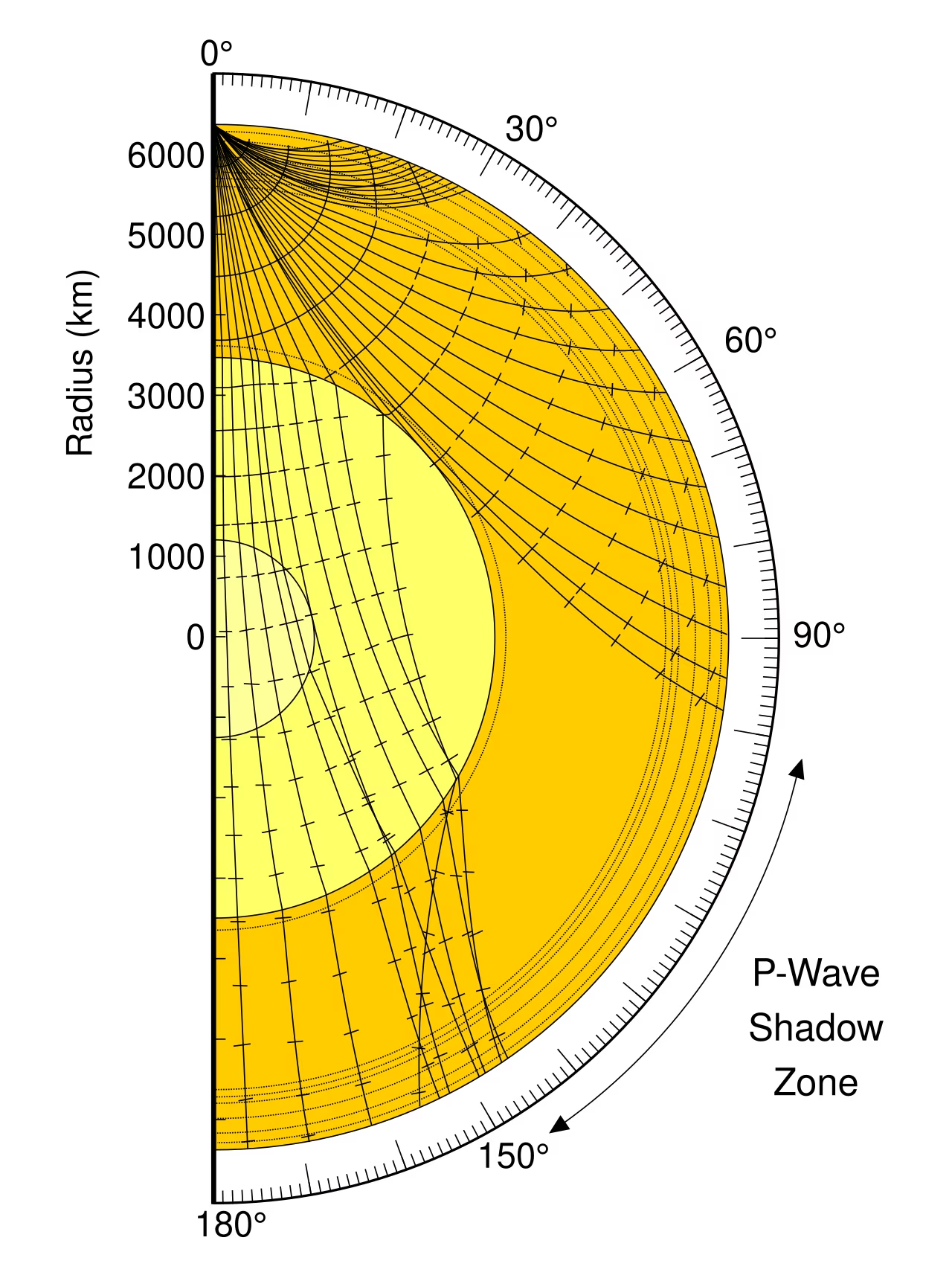
Fig. 8.1 Ray paths of seismic P-waves through Earth’s interior, with the radius in km and the angular distance from the source on the rim. Rays refract continuously through the mantle; those that enter the liquid outer core bend sharply downward because the P-wave speed drops at the core-mantle boundary, so no direct P arrival reaches the surface between about 103° and 143° from the source, the P-wave shadow zone. S-waves (not shown) do not cross the liquid core at all. Credit: Wikimedia Commons, public domain.

The geometry follows from a single conserved quantity. In a spherically symmetric body the ray parameter

\[ p = \frac{r \sin i}{v(r)} \]

is constant along a ray, where \(i\) is the angle between the ray and the local radial direction. A ray bottoms out at the radius where \(r/v(r) = p\), and its angular distance is

\[ \Delta = 2 \int_{r_{\rm turn}}^{R} \frac{p \, \mathrm{d}r}{r \sqrt{\left(r/v\right)^2 - p^2}} . \]

Integrating this through PREM, the reference model of Earth’s radial structure presented in the section on Earth’s interior, reproduces the observed shadow zones without any free parameters.

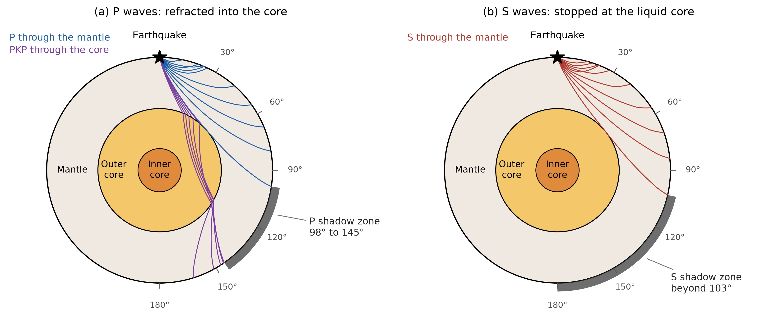
Fig. 8.2 Seismic rays traced through the PREM velocity model for a surface source. (a) P-waves. Rays that bottom in the mantle emerge no further than 98° from the source, because compressional wave speed drops from 13.7 to 8.1 km s\(^{-1}\) across the core-mantle boundary; rays that enter the outer core are bent sharply downward and return only beyond the PKP caustic at 145°. The shaded arc is the resulting P-wave shadow zone. (b) S-waves. Shear waves do not propagate through a liquid, so every S ray bottoms in the mantle and none arrives beyond 103°. The classical values quoted in textbooks, 103° to 143°, are slightly narrower at the near edge because waves diffracted along the core-mantle boundary extend the direct branch by a few degrees. Faint arrivals refracted through the solid inner core (PKIKP) return into the P shadow zone from about 116°, which is how the inner core was identified. Course-original figure.

Gravity field measurements constrain the distribution of mass within a planet. A perfectly spherical, homogeneous body produces a purely \(1/r^2\) gravitational field. Real planets are oblate due to rotation, producing a measurable gravitational quadrupole moment \(J_2\), the leading correction to the field beyond a simple \(1/r^2\) dependence. The value of \(J_2\) depends on how mass is distributed between the equator and the poles, which in turn depends on the density profile. Higher-order gravity harmonics reveal lateral density variations. Spacecraft in orbit (e.g., GRAIL at the Moon, Juno at Jupiter) measure gravity fields with extraordinary precision by tracking tiny Doppler shifts in their radio signals.

The moment of inertia is perhaps the single most diagnostic quantity for constraining a planet’s internal mass distribution. For a body of mass \(M\) and radius \(R\), the dimensionless moment of inertia factor \(C/MR^2\) (where \(C\) is the polar moment of inertia) ranges from \(2/5 = 0.4\) for a uniform-density sphere to lower values for bodies with mass concentrated toward the centre (Fig. 8.4). A measured value immediately tells us the degree of differentiation, the extent to which an initially more uniform body has separated into compositionally distinct layers, such as a dense metallic core and a lighter silicate mantle, through melting and gravitational settling:

Body	\(C/MR^2\)	Interpretation
Uniform sphere	0.400	Reference value (\(2/5\))
Moon	0.393	Weakly differentiated, small core
Mars	0.364	Moderately differentiated
Mercury	0.346	Large dense core
Earth	0.331	Strongly differentiated, iron core

Fig. 8.3 shows why differentiation lowers the factor: at fixed outer radius, moving mass into a dense central core removes it from large distances to the rotation axis, which suppresses the moment of inertia \(C\) more strongly than the mass \(M\).

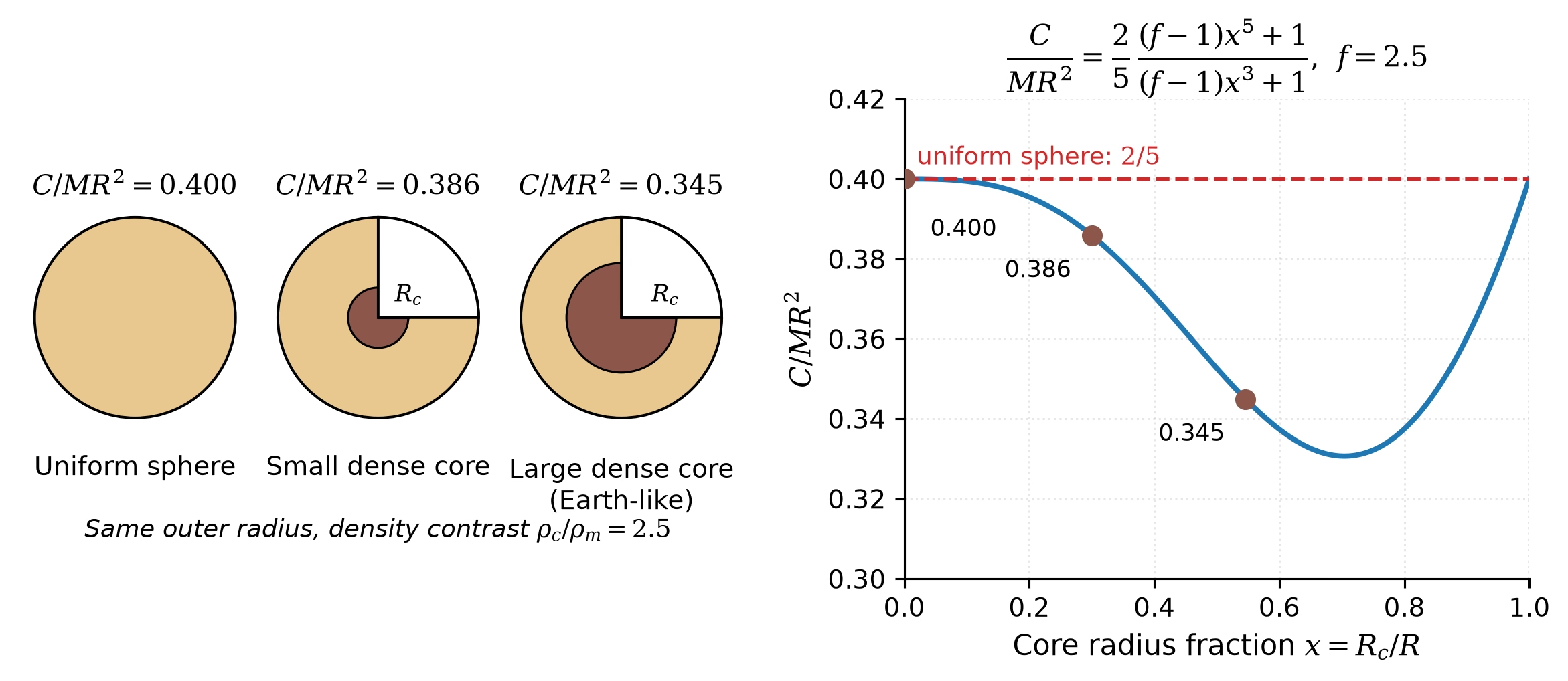
Fig. 8.3 Central mass concentration and the moment of inertia factor. Left: cutaway views of three two-layer spheres with the same outer radius and a fixed core-to-mantle density contrast \(\rho_c/\rho_m = 2.5\), differing only in the core radius fraction \(x = R_c/R\); the quoted \(C/MR^2\) values follow from the two-layer relation (8.3) derived in the blackboard section below. Right: the same relation as a continuous function of \(x\), with the three configurations marked. The factor falls below the uniform-sphere value \(2/5\) as soon as a dense core forms, and the \(x = 0.546\) case reproduces the Earth-like worked example of the derivation. The curve climbs back to \(0.4\) as \(x \to 1\), where the body is again a uniform sphere, now made entirely of core material. Course-original figure.

The moment of inertia factor is determined observationally from two quantities: the gravitational oblateness \(J_2\) (from spacecraft tracking) and the precession rate of the spin axis (or, equivalently, the forced libration amplitude, the small periodic oscillation of a body’s orientation about its mean rotation, for bodies in spin-orbit resonance, i.e. rotating at a simple integer ratio to their orbital period). These are combined using the Darwin-Radau relation, which relates \(C/MR^2\) to \(J_2\) and the rotational flattening.

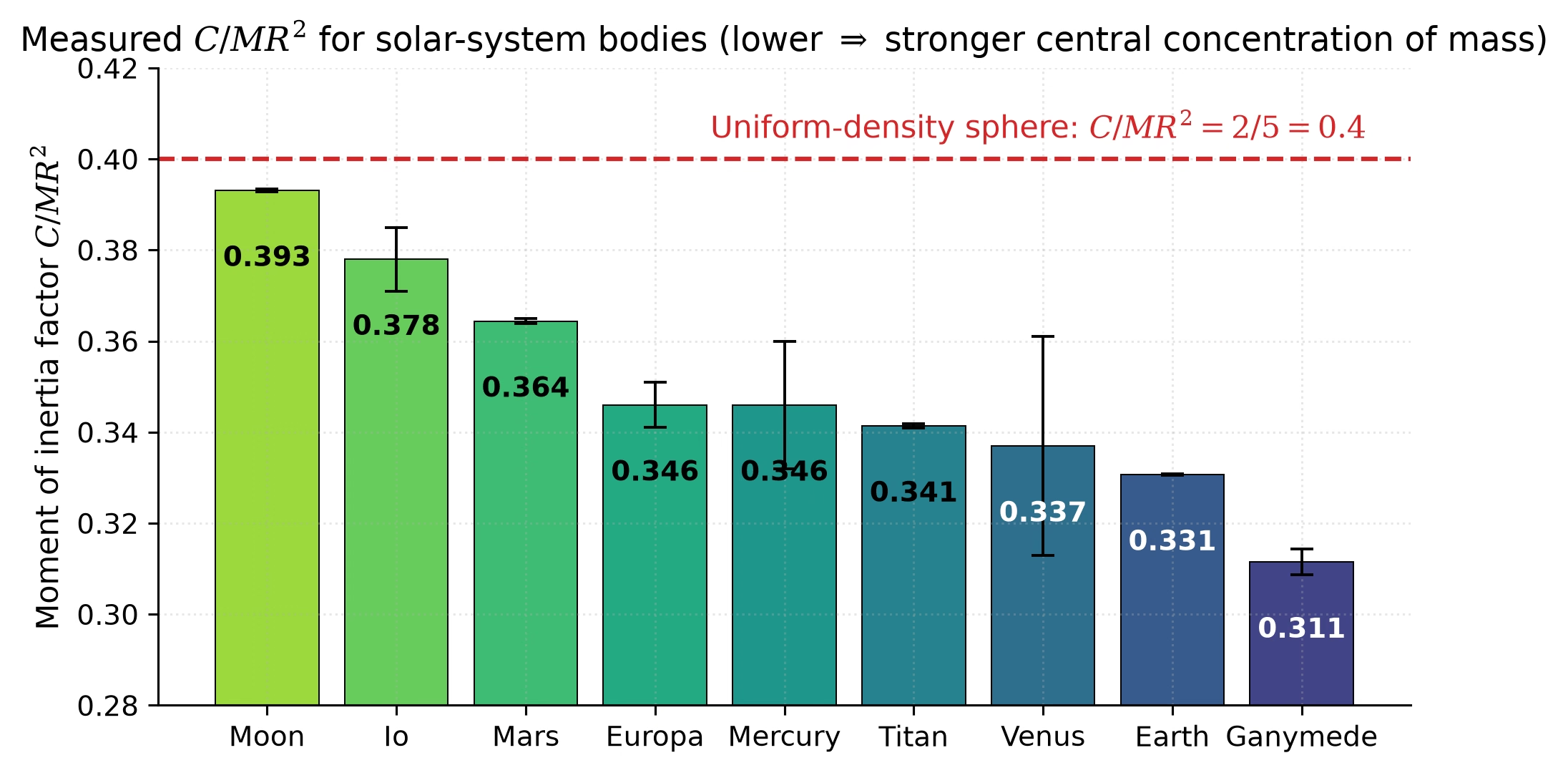
Fig. 8.4 Measured moment of inertia factors \(C/MR^2\) for nine solar-system bodies. The dashed red line marks the value \(2/5 = 0.4\) for a uniform-density sphere. Lower values indicate stronger central concentration of mass: the Moon (\(C/MR^2 = 0.393\)) is only weakly differentiated, whereas Earth (\(0.331\)) and Ganymede (\(0.311\)) are strongly differentiated bodies with dense iron or iron-sulfide cores. Earth value from PREM; lunar value from combined GRAIL gravity and lunar laser ranging [Williams et al., 2014]; Mars, Mercury, and outer-planet satellite values are standard literature compilations. Uniform-sphere value from elementary mechanics. Course-original figure.

8.2. Blackboard derivation: Moment of inertia factor

Blackboard derivation: \(C/MR^2\) for uniform and differentiated bodies

Goal: Derive the moment of inertia factor for (a) a uniform sphere and (b) a two-layer differentiated body, and show how the measured value constrains internal structure.

Step 1: Moment of inertia of a spherically symmetric body.

The moment of inertia about the rotation axis is \(C = \int r_\perp^2 \, dm\), where \(r_\perp\) is the perpendicular distance from the axis. For a thin spherical shell of radius \(r\) and density \(\rho(r)\), the moment of inertia about a diameter is \(dC = \frac{2}{3}r^2 \, dm\), where \(dm = 4\pi r^2 \rho(r) \, dr\) (Fig. 8.5). Integrating over all shells:

(8.1)\[ C = \frac{8\pi}{3} \int_0^R \rho(r) \, r^4 \, dr \]

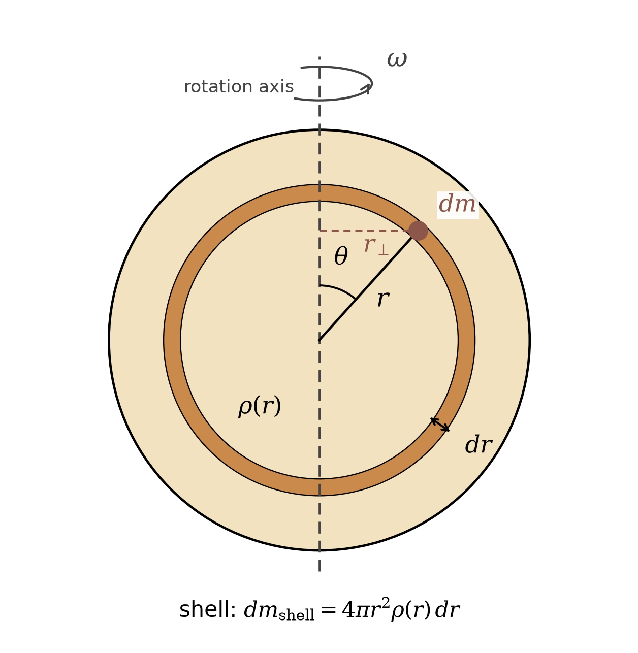
Fig. 8.5 The geometry behind (8.1). The body spins about the vertical axis at rate \(\omega\). A mass element \(dm\) at radius \(r\) and colatitude \(\theta\) sits at perpendicular distance \(r_\perp = r\sin\theta\) from the axis and contributes \(r_\perp^2\,dm\) to \(C\). A thin shell of radius \(r\) and thickness \(dr\) (shaded) carries the mass \(4\pi r^2 \rho(r)\,dr\), and \(\sin^2\theta\) averages to \(2/3\) over the surface of a sphere, which gives \(dC = \frac{2}{3}r^2\,dm\) and, integrated over all shells, (8.1). Course-original figure.

Step 2: Uniform sphere (\(\rho = \text{const}\)).

\[ C = \frac{8\pi}{3} \rho \int_0^R r^4 \, dr = \frac{8\pi}{3} \rho \frac{R^5}{5} = \frac{8\pi}{15} \rho R^5 \]

Using \(M = \frac{4}{3}\pi R^3 \rho\):

(8.2)\[ \boxed{\frac{C}{MR^2} = \frac{8\pi\rho R^5 / 15}{(4\pi\rho R^3/3)\,R^2} = \frac{2}{5} = 0.400} \]

Step 3: Two-layer body with a dense core (density \(\rho_c\), radius \(R_c\)) and lighter mantle (density \(\rho_m\), extending from \(R_c\) to \(R\)):

\[ C = \frac{8\pi}{15} \left[ (\rho_c - \rho_m)\,R_c^5 + \rho_m\,R^5 \right] \]

\[ M = \frac{4}{3}\pi \left[ (\rho_c - \rho_m)\,R_c^3 + \rho_m\,R^3 \right] \]

Defining \(x \equiv R_c/R\) and \(f \equiv \rho_c/\rho_m\):

(8.3)\[ \boxed{\frac{C}{MR^2} = \frac{2}{5} \cdot \frac{(f-1)\,x^5 + 1}{(f-1)\,x^3 + 1}} \]

When \(f > 1\) (dense core), the factor multiplying \(2/5\) is less than 1, because \(x^5 < x^3\) for \(0 < x < 1\). Concentrating mass toward the centre pulls \(C/MR^2\) below the uniform-sphere value of 0.4. The effect is strongest at intermediate core sizes: as \(x \to 1\) the body is again nearly uniform, and the factor climbs back toward 0.4.

Worked example: Earth. With \(R_c/R \approx 3480/6371 \approx 0.546\) and \(\rho_c/\rho_m \approx 11{,}000/4{,}400 \approx 2.5\):

\[ \frac{C}{MR^2} = \frac{2}{5} \times \frac{1.5 \times 0.049 + 1}{1.5 \times 0.163 + 1} = 0.4 \times \frac{1.073}{1.244} \approx 0.345 \]

The measured value is \(C/MR^2 = 0.3307\), close to our two-layer estimate, with the remaining difference due to the continuous density increase within each layer (PREM gives an additional \(\sim 5\%\) density jump across the inner-core boundary).

Key insight: A single number, \(C/MR^2\), immediately distinguishes an undifferentiated rubble pile (0.4) from a strongly differentiated body like Earth (0.33). This is often the first constraint available for a newly characterised planet or moon.

Fig. 8.6 sorts the five bodies by this factor.

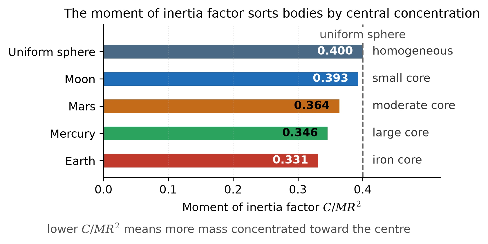
Fig. 8.6 The moment of inertia factor \(C/MR^2\) for a uniform sphere (0.400), the Moon (0.393), Mars (0.364), Mercury (0.346) and Earth (0.331): a lower value means more mass concentrated toward the centre, from a homogeneous body to one with a large iron core. Values after de Pater and Lissauer (2010). Course-original figure.

8.3. Equations of state

To construct a quantitative model of a planetary interior, we need an equation of state (EOS) that relates pressure \(P\), density \(\rho\), and temperature \(T\) at every depth. The starting point is hydrostatic equilibrium: the condition that pressure at each depth supports the weight of the overlying material. In spherical symmetry [Turcotte and Schubert, 2002]:

(8.4)\[ \frac{dP}{dr} = -\rho(r)\,g(r) = -\frac{G\,m(r)\,\rho(r)}{r^2} \]

where \(m(r) = 4\pi\int_0^r \rho(r')\,r'^2\,dr'\) is the mass enclosed within radius \(r\) and \(g(r) = Gm(r)/r^2\) is the local gravitational acceleration. This equation, combined with an EOS, can be integrated inward from the surface to determine the pressure, density, and composition at every depth.

For a rough estimate of the central pressure of a planet, we can assume uniform density \(\bar{\rho} = 3M/(4\pi R^3)\):

(8.5)\[ P_c \approx \frac{3\,G\,M^2}{8\pi\,R^4} \]

For Earth (\(M = 5.97 \times 10^{24}\) kg, \(R = 6371\) km), this gives \(P_c \approx 170\) GPa, roughly half the actual value of \(\sim\)360 GPa, because the real density increases substantially toward the centre [Dziewonski and Anderson, 1981]. Fig. 8.7 extends this comparison across the solar system: every body plots above the line of equality, and the gap grows from a few per cent for the nearly homogeneous Moon to a factor of about three for Jupiter, whose deep interior is both strongly compressed and centrally condensed.

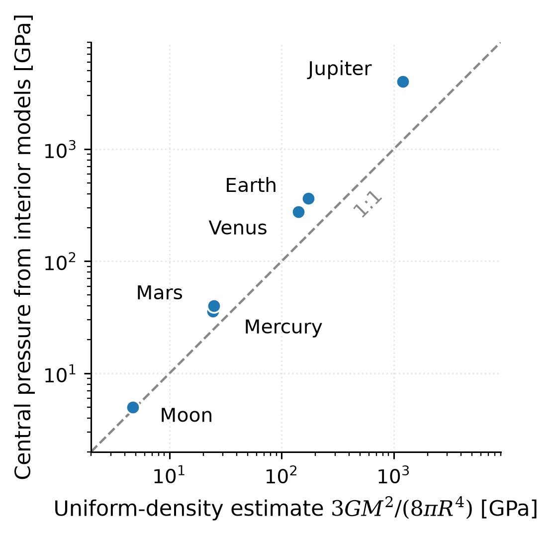
Fig. 8.7 Central pressure from interior models against the uniform-density estimate of (8.5) for six solar-system bodies, on logarithmic axes. The dashed line marks equality: a body of uniform density would fall on it. All bodies sit above the line because density increases toward the centre; the offset grows from a few per cent for the Moon to a factor of about three for Jupiter. Model central pressures: Moon [Weber et al., 2011], Mercury [Margot et al., 2018], Mars [Stähler et al., 2021] (see text for the 2023 core-boundary revision), Venus [Aitta, 2012], Earth [Dziewonski and Anderson, 1981], Jupiter [Wahl et al., 2017]. Course-original figure.

The simplest equation of state in physics is the ideal gas law, \(P = \rho\,k_B T/(\mu m_u)\), where \(\mu\) is the mean molecular mass in atomic mass units. It describes planetary atmospheres well, where pressure is thermal: particle momentum flux sets density in direct proportion to \(P\) and inverse proportion to \(T\). Planetary interiors are condensed matter where the ideal gas law fails completely. In rock, iron, or ice the interatomic spacing is set by electrostatic attraction and quantum-mechanical repulsion of overlapping electron shells (several electronvolts per atom), whereas thermal energy at mantle temperatures is only \(k_B T \approx 0.2\) eV at 2000 K. Pressure in a solid or liquid planet is therefore elastic rather than thermal: compressing rock requires tens of gigapascals, and density depends only weakly on temperature. At lower-mantle conditions (\(P \approx 100\) GPa, \(T \approx 2500\) K, \(\mu \approx 20\) for MgSiO\(_3\)), the ideal gas law predicts \(\rho \approx 10^5\) kg m\(^{-3}\), roughly twenty times the true \(\sim\)5000 kg m\(^{-3}\); at Earth’s surface (\(P = 1\) bar, \(T = 300\) K) it predicts \(\rho \approx 1\) kg m\(^{-3}\), three thousand times too low. Planetary interiors therefore require equations of state built for condensed matter, anchored in laboratory compression experiments and quantum-mechanical calculations.

Fig. 8.8 shows what such condensed-matter equations of state look like for the three canonical planet-building materials: iron, silicate (MgSiO\(_3\)), and water, drawn from the PALEOS multiphase EOS framework [Attia et al., 2026]. First, condensed matter is stiff: along the 300 K isotherm each material must be squeezed to tens of gigapascals before its density rises appreciably, and even at \(10^4\) GPa, deep-giant-planet pressure, iron is compressed only five-fold. Second, density does not rise smoothly: discrete steps mark phase transitions to more densely packed crystal structures (\(\alpha\)- to \(\varepsilon\)-iron; enstatite through bridgmanite to post-perovskite in the silicate; high-pressure ices VII and X in water), some of which appear as seismic discontinuities inside Earth (Phase transitions). Third, temperature matters only where pressure is low: heating iron from 300 to 4000 K lowers its density by 12 per cent at 0.1 GPa but by only 2 per cent at Earth’s central pressure, where compression dominates. Water is the instructive exception: at 4000 K and low pressure it is a supercritical fluid twenty times less dense than the cold liquid; its hot and cold branches still differ by more than 10 per cent at 100 GPa and converge to the few-per-cent level only near Earth’s central pressure. Equations of state like these are the foundation on which mass-radius relations for exoplanets are built Lecture 13.

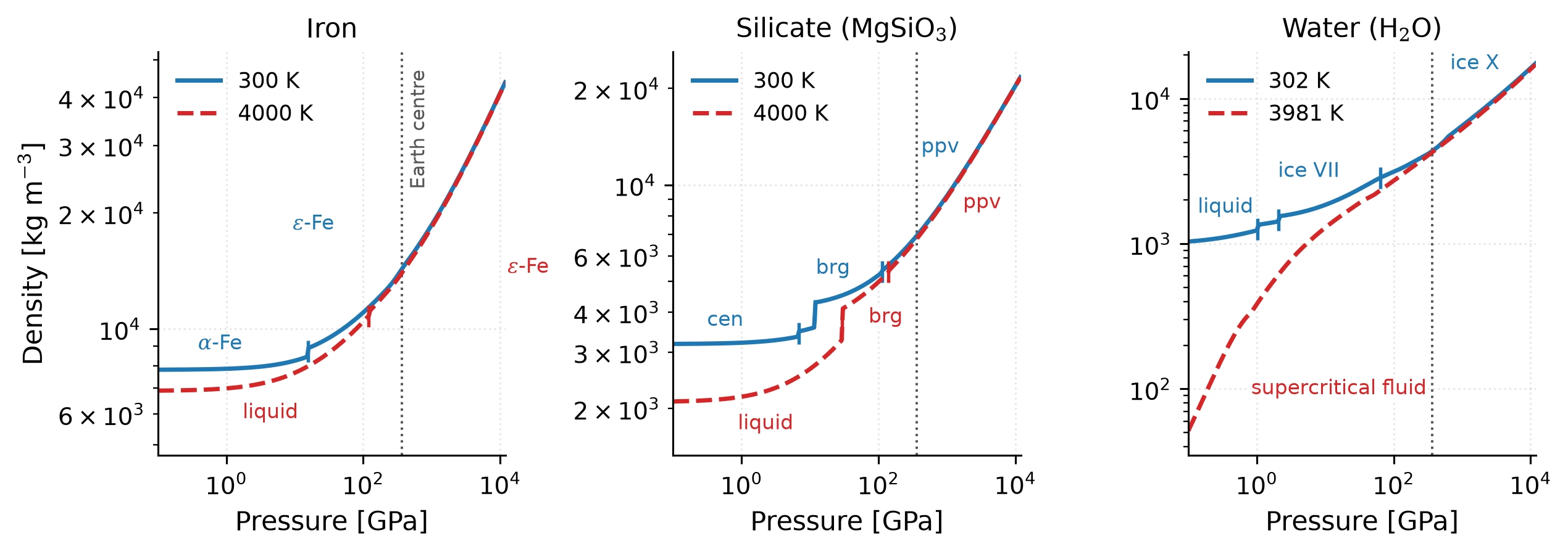
Fig. 8.8 Density as a function of pressure for iron, silicate (MgSiO\(_3\)), and water from the PALEOS multiphase equation-of-state tables [Attia et al., 2026]. Each panel compares a cold (solid blue) and a hot (dashed red) isotherm at the tabulated temperatures nearest 300 and 4000 K (302 and 3981 K for water); short vertical bars and labels mark the stable phase along each curve, and the dotted vertical line marks Earth’s central pressure (\(\sim\)364 GPa). At low pressure the isotherms differ, most dramatically for water, where the hot branch is a low-density supercritical fluid; with increasing pressure compression overwhelms thermal expansion and the curves converge, for iron and silicate by \(\sim\)100 GPa, for water only near Earth’s central pressure. Course-original figure from the tabulated data of Attia et al. [2026].

At the pressures and temperatures found in planetary interiors (\(P \sim 1\)–\(10^4\) GPa, \(T \sim 10^3\)–\(10^4\) K), material behaviour differs drastically from surface conditions. The bulk modulus \(K = -V\,dP/dV = \rho\,dP/d\rho\) describes a material’s resistance to compression. Birch [1952] established an empirical relationship between compressional wave velocity \(v_P\) and density for silicates and oxides (Fig. 8.9), known as Birch’s law, which remains a cornerstone of mineral physics.

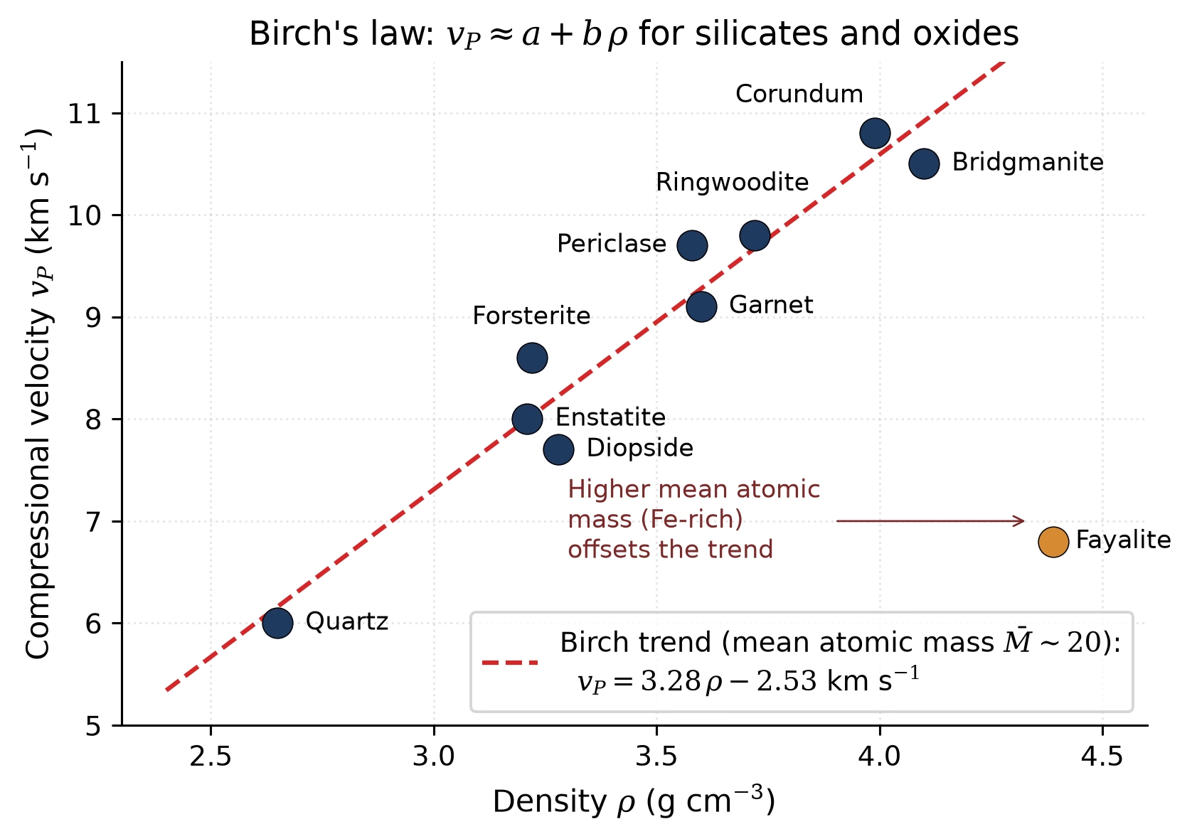
Fig. 8.9 Birch’s law for silicates and oxides: compressional-wave velocity \(v_P\) plotted against density \(\rho\) for common mantle-forming minerals at ambient conditions. The approximately linear trend (red dashed) holds at fixed mean atomic mass and allows seismic velocities measured at depth to be mapped to densities, provided the composition (mean atomic mass) is known. Outliers such as Fe-rich fayalite sit below the main trend because their higher mean atomic mass reduces \(v_P\) at a given density. Mineral values from standard mineral-physics compilations. Trend originally established by Birch [1952]. Course-original figure.

The seismic parameter \(\phi \equiv K_S/\rho = v_P^2 - \frac{4}{3}v_S^2\) (where \(K_S\) is the adiabatic bulk modulus) connects seismological observables directly to the EOS. The Adams-Williamson equation uses this to relate the density gradient to the seismic velocities:

\[ \frac{d\rho}{dr} = -\frac{\rho(r)\,g(r)}{\phi(r)} \]

This equation allows seismologists to determine the density profile from measured wave speeds, provided the composition is approximately uniform within each layer and temperature effects are small. Tested against the Preliminary Reference Earth Model (PREM), the standard radial profile of Earth’s density and seismic wave speeds assembled from global earthquake data [Dziewonski and Anderson, 1981] and presented in detail in the next section, the Adams-Williamson relation reproduces the smooth lower-mantle density rise from self-compression alone but breaks down at the core-mantle boundary, where a discontinuous density jump signals the compositional change from silicate mantle to iron-alloy core (Fig. 8.10).

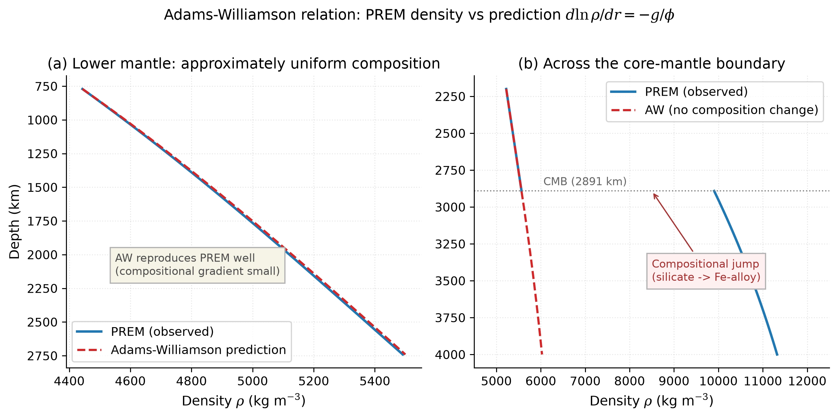
Fig. 8.10 Test of the Adams-Williamson relation against PREM. (a) In the lower mantle (771-2741 km depth), where composition is approximately uniform, the density predicted by integrating \(d\ln\rho/dr = -g/\phi\) (red dashed) reproduces the observed PREM profile (blue) closely: the density rise is dominated by self-compression. (b) Across the core-mantle boundary at 2891 km depth, the observed density (blue) jumps discontinuously from \(\sim\)5570 to \(\sim\)9900 kg m\(^{-3}\), whereas a no-composition-change Adams-Williamson extrapolation (red dashed) predicts a smooth, far smaller increase. The deviation directly exposes the compositional change from silicate mantle to iron-alloy core. Course-original figure from the PREM tabulation of Dziewonski and Anderson [1981].

8.4. Earth’s interior

Earth is the best-characterised planetary interior, thanks to thousands of seismometers recording earthquakes worldwide. The Preliminary Reference Earth Model (PREM; [Dziewonski and Anderson, 1981]) synthesises travel-time data from millions of seismic arrivals into radial profiles of density, elastic moduli, and wave speeds (Fig. 8.11, Fig. 8.12). Earth’s interior consists of four major layers:

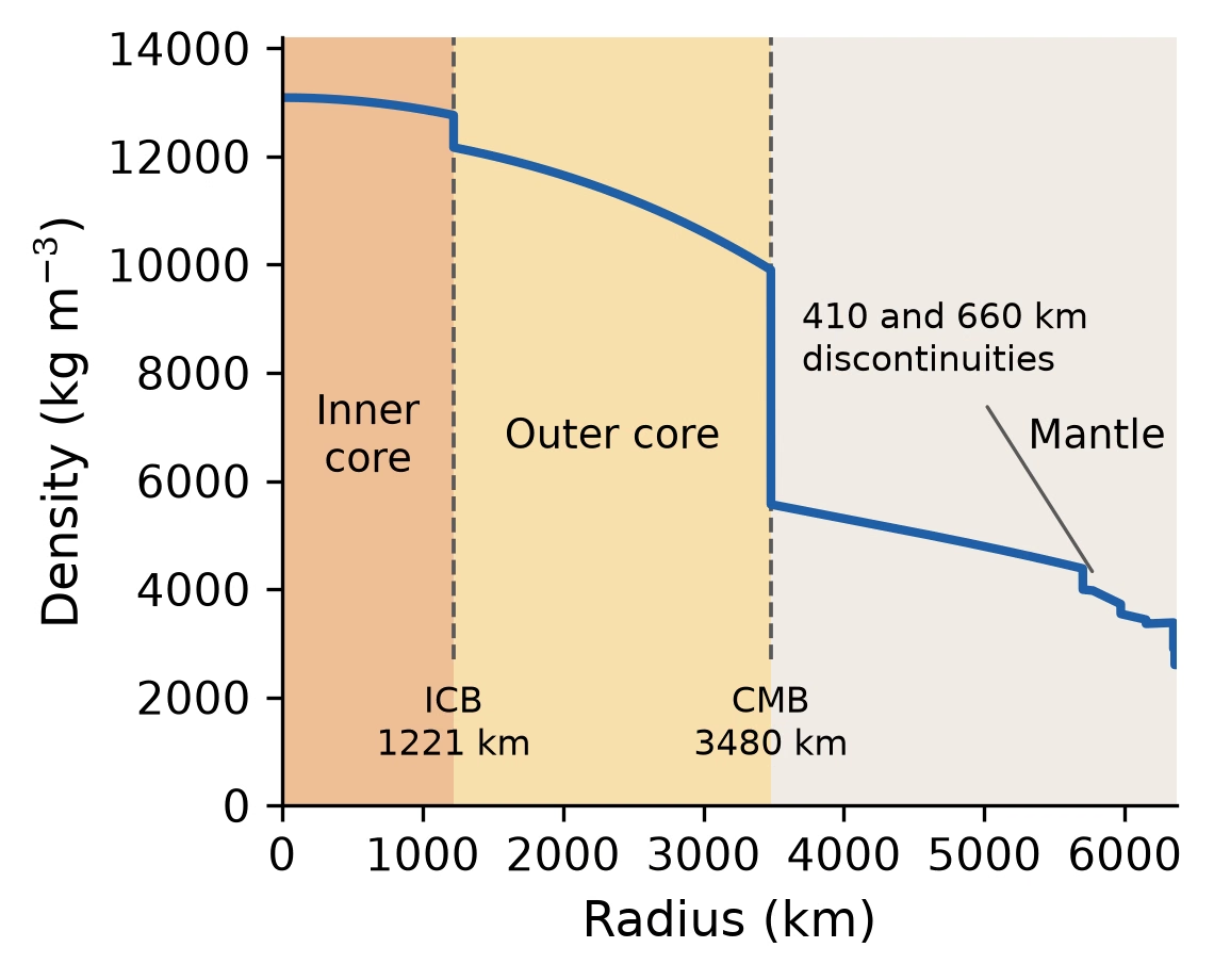
Fig. 8.11 The Preliminary Reference Earth Model (PREM) density profile as a function of radius, evaluated directly from the polynomial coefficients of Dziewonski and Anderson [1981]. The density increases from \(\sim\)3300 kg m\(^{-3}\) in the upper mantle to \(\sim\)5570 kg m\(^{-3}\) at the base of the mantle, then jumps sharply at the core-mantle boundary (CMB, 3480 km radius) to \(\sim\)9900 kg m\(^{-3}\) in the outer core. The inner core boundary at 1221 km radius marks another increase, from 12,170 to 12,760 kg m\(^{-3}\), and the density reaches 13,090 kg m\(^{-3}\) at the centre. The two smaller steps near the top of the mantle are the 410 and 660 km discontinuities, where mineral phase transitions raise the density at constant bulk composition. Each PREM branch is sampled on its own interval, so every discontinuity appears as a vertical riser rather than a smoothed ramp. Course-original figure.

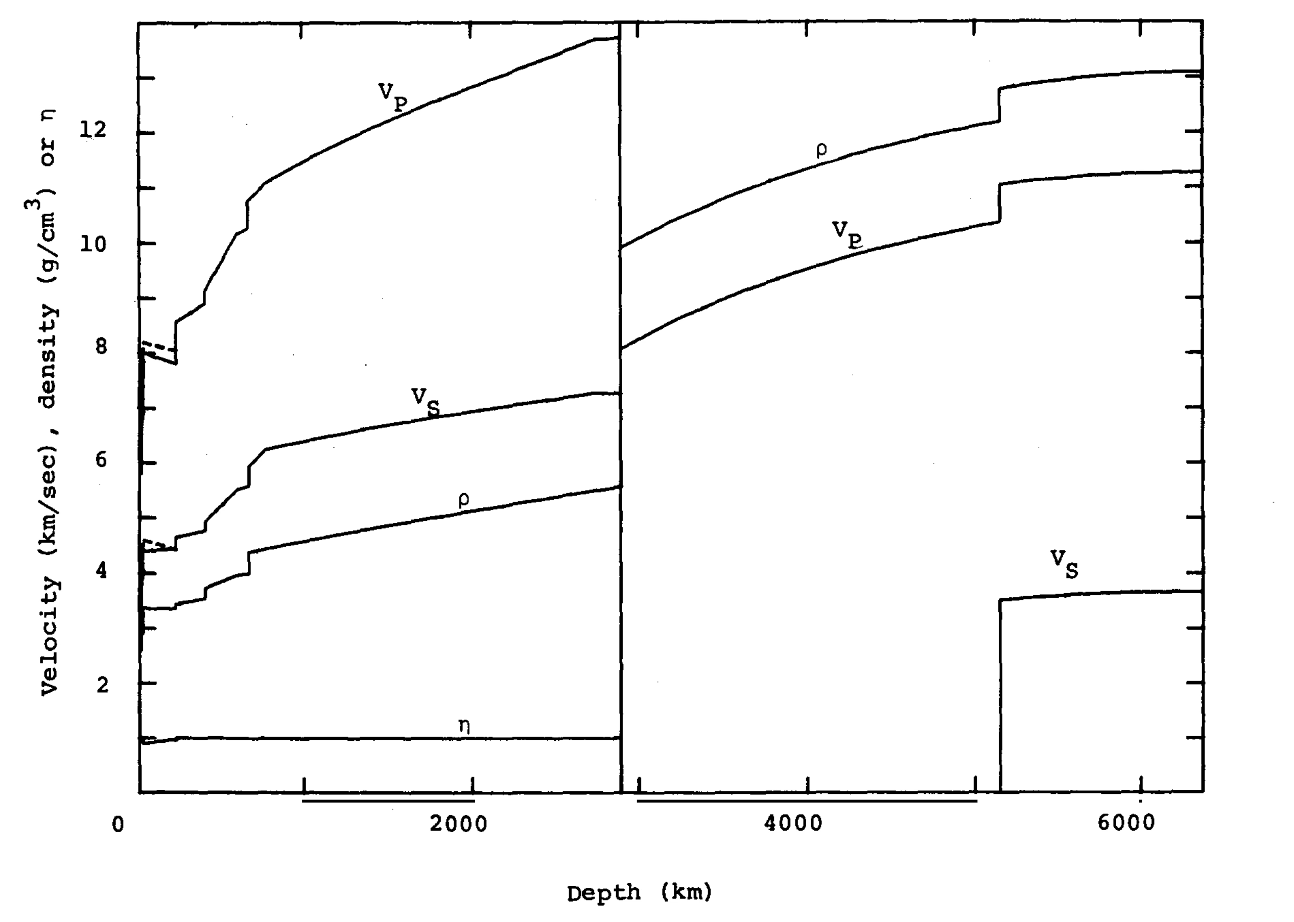
Fig. 8.12 PREM radial profiles of compressional (\(v_P\)) and shear (\(v_S\)) wave speeds, density (\(\rho\), in g cm\(^{-3}\)), and the anisotropy parameter \(\eta\) as functions of depth. A vertical break at the core-mantle boundary (\(\sim\)2890 km) divides the panel: the mantle on the left, with the finely structured uppermost mantle and transition zone compressed against the left axis, and the core on the right. Dashed curves in the upper mantle are the horizontal velocity components, so their separation from the solid curves measures the anisotropy there; \(\eta\) stays near unity elsewhere. In the liquid outer core \(v_S\) is absent, and it reappears at the inner-core boundary near 5150 km depth where the solid inner core begins. Reproduced from [Dziewonski and Anderson, 1981], Fig. 8.

The crust is Earth’s outermost solid layer, varying from \(\sim\)5–10 km thick beneath the oceans (dense basaltic rock, \(\rho \approx 3000\) kg m\(^{-3}\)) to \(\sim\)30–70 km thick beneath the continents (lighter granitic rock, \(\rho \approx 2700\) kg m\(^{-3}\)). Despite being the layer we inhabit and study most directly, the crust constitutes less than 1% of Earth’s total mass.

The mantle extends from the base of the crust (the Mohorovičić discontinuity, or Moho) down to 2891 km depth. It is composed primarily of silicate minerals rich in magnesium and iron. Key seismic discontinuities divide it into:

• Upper mantle (to ~410 km): dominated by olivine (\(\mathrm{(Mg,Fe)_2SiO_4}\)), with densities of 3300–3700 kg m\(^{-3}\)

• Transition zone (410–660 km): olivine transforms to higher-pressure polymorphs, denser crystal structures of the same chemical composition (wadsleyite, then ringwoodite; see Phase transitions below)

• Lower mantle (660–2891 km): dominated by bridgmanite (\(\mathrm{(Mg,Fe)SiO_3}\)) and ferropericlase (\(\mathrm{(Mg,Fe)O}\)), with densities reaching \(\sim\)5570 kg m\(^{-3}\) at the base

The outer core (2891–5150 km depth) is a liquid alloy of iron and nickel with \(\sim\)10% lighter elements (likely sulfur, oxygen, silicon, or hydrogen). Its liquid state is proven by the absence of S-waves and by the existence of Earth’s magnetic dynamo (Lecture 4), which requires a convecting, electrically conducting fluid. Temperatures range from \(\sim\)4000 K at the top to \(\sim\)5000 K at the base.

The inner core (5150–6371 km depth) is solid iron-nickel, crystallised from the cooling outer core. Despite temperatures of \(\sim\)5000–6000 K, the enormous pressure (\(\sim\)330–360 GPa) keeps it solid. The inner core grows at an estimated rate of \(\sim\)0.5 mm yr\(^{-1}\) as Earth slowly cools, and the latent heat released by this crystallisation is an important energy source for driving the geodynamo [Schubert et al., 2001]. Fig. 8.13 draws these four layers to scale.

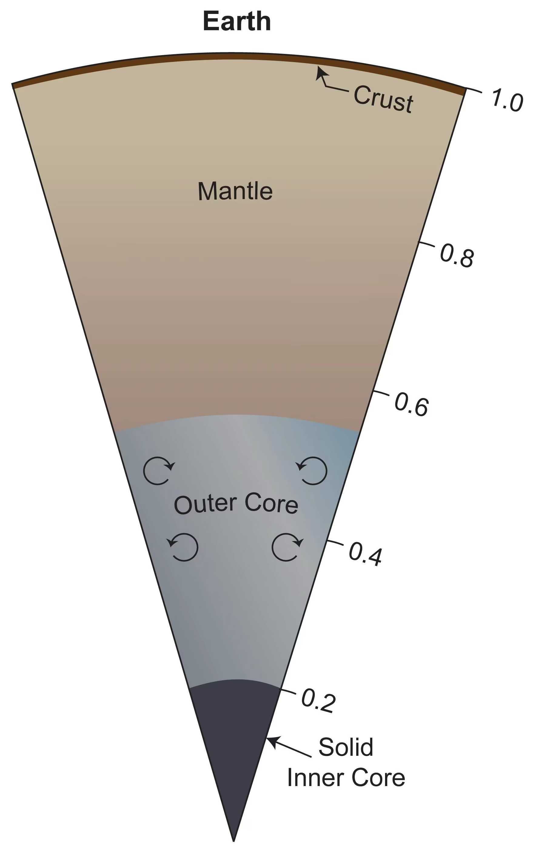
Fig. 8.13 Earth’s internal structure shown as a radial cross-section. The thin crust (brown) overlies the silicate mantle, which reaches down to about 0.55 of Earth’s radius. Below lies the liquid outer core (with convection currents driving the geodynamo, the process by which motion of an electrically conducting fluid generates a planetary magnetic field) and the solid inner core at the centre. The fractional radius scale on the right shows how the core occupies roughly the inner 55% of Earth by radius. Credit: NASA/JPL-Caltech/SwRI/John E. Connerney (PIA25063).

8.5. Mantle rheology

Although Earth’s mantle is solid (it transmits S-waves), it flows over geological timescales. This seemingly paradoxical behaviour arises because the mantle’s viscosity (a measure of resistance to flow) is finite, around \(10^{21}\) Pa·s for the upper mantle (compare \(\sim\)10\(^{-3}\) Pa·s for water and \(\sim\)10\(^{12}\) Pa·s for glacial ice). At temperatures above roughly half the melting point, solid-state creep mechanisms allow crystals to deform slowly by the diffusion of atoms along grain boundaries or through the crystal lattice [Karato, 2008].

Whether the mantle convects vigorously is governed by the Rayleigh number (introduced in Lecture 3):

\[ \text{Ra} = \frac{\alpha\,\rho\,g\,\Delta T\,d^3}{\kappa\,\eta} \]

where \(\alpha\) is the thermal expansivity, \(\Delta T\) the temperature difference driving convection, \(d\) the layer thickness, \(\kappa\) the thermal diffusivity, and \(\eta\) the dynamic viscosity. For Earth’s mantle, \(\text{Ra} \sim 10^7\)–\(10^8\), far above the critical value \(\text{Ra}_c \approx 10^3\), so the mantle convects vigorously, driving plate tectonics at the surface Lecture 7.

The pattern of mantle convection was long framed as a dichotomy (Fig. 8.14). Whole-mantle convection models have material circulating from the surface to the core-mantle boundary, while layered convection models propose that the 660 km discontinuity impedes flow, creating separate upper- and lower-mantle circulation cells. Seismic tomography (imaging the mantle’s 3D velocity structure) has since resolved the central question: cold subducted slabs can be traced from subduction zones deep into the lower mantle, with some slab segments apparently sinking to the base of the mantle [van der Hilst et al., 1997], and broad low-velocity conduits rise from the core-mantle boundary beneath major hotspots [French and Romanowicz, 2015]. Mass evidently crosses the 660 km boundary in both directions, so strictly layered convection is no longer tenable.

The boundary still shapes the flow, however. Global tomographic surveys show that slab behaviour at 660 km varies regionally: some slabs penetrate directly into the lower mantle, others flatten and stagnate above the discontinuity, and others are trapped between 660 and 1000 km depth before resuming their descent [Fukao and Obayashi, 2013]. The debate continues over the nature and longevity of chemical heterogeneity within a whole-mantle circulation.

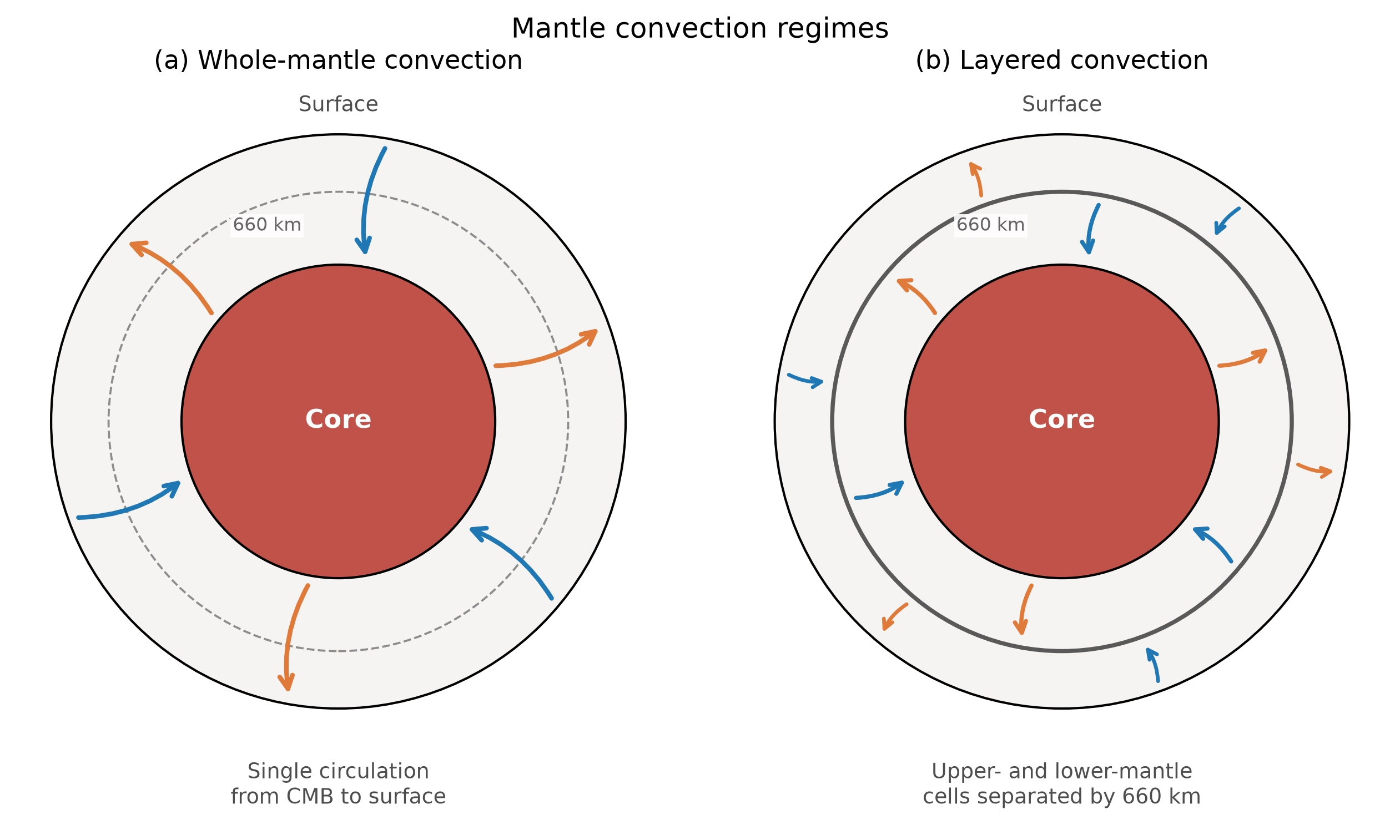
Fig. 8.14 End-member regimes of mantle convection. (a) Whole-mantle convection: a single circulation pattern carries material from the core-mantle boundary all the way to the surface, and the arrows cross the 660 km discontinuity, drawn dashed because it only weakly impedes the flow; the boundary radii are not to scale. (b) Layered convection: separate cells operate above and below the boundary, drawn solid because it blocks the flow, decoupled by the negative Clapeyron slope (the pressure of the phase boundary decreases as temperature increases) of the ringwoodite-to-bridgmanite phase transition at 660 km. Both end members are idealisations: seismic tomography shows slabs crossing the boundary in some subduction zones and stagnating above it in others, favouring whole-mantle circulation with regionally variable resistance at 660 km [Fukao and Obayashi, 2013]. Schematic; not to scale, and the radius of the 660 km boundary is exaggerated so that a circulation cell fits above it. Course-original figure.

Fig. 8.15 places the two creep mechanisms on the viscosity axis, and Fig. 8.16 shows how far Earth’s mantle sits above the onset of convection, and how much faster than conduction it moves heat.

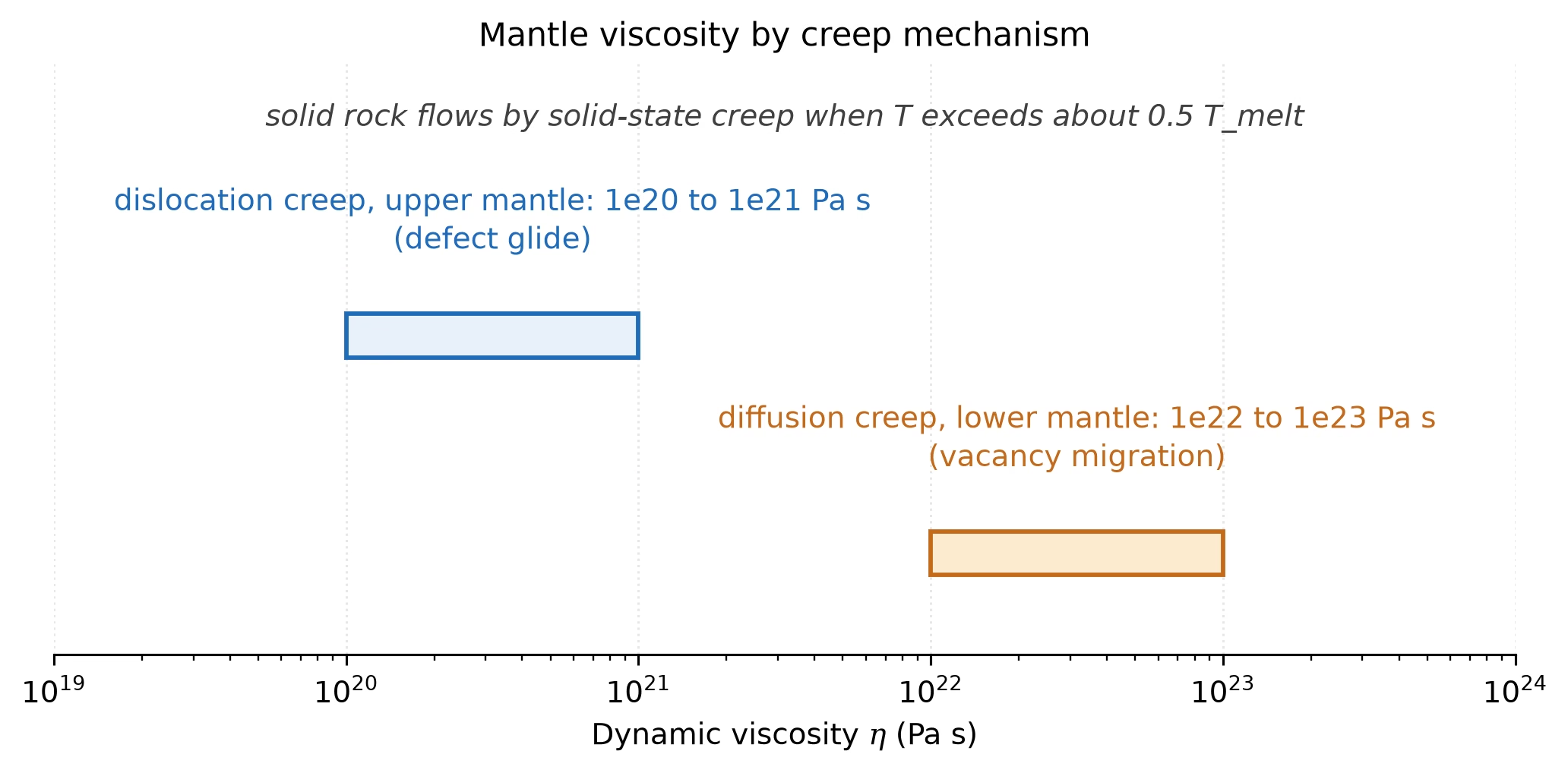
Fig. 8.15 Mantle viscosity by creep mechanism: dislocation creep (defect glide) dominates the upper mantle at \(10^{20}\) to \(10^{21}\) Pa s, diffusion creep (vacancy migration) the lower mantle at \(10^{22}\) to \(10^{23}\) Pa s; solid rock flows by solid-state creep once the temperature exceeds about half the melting temperature. Course-original figure.

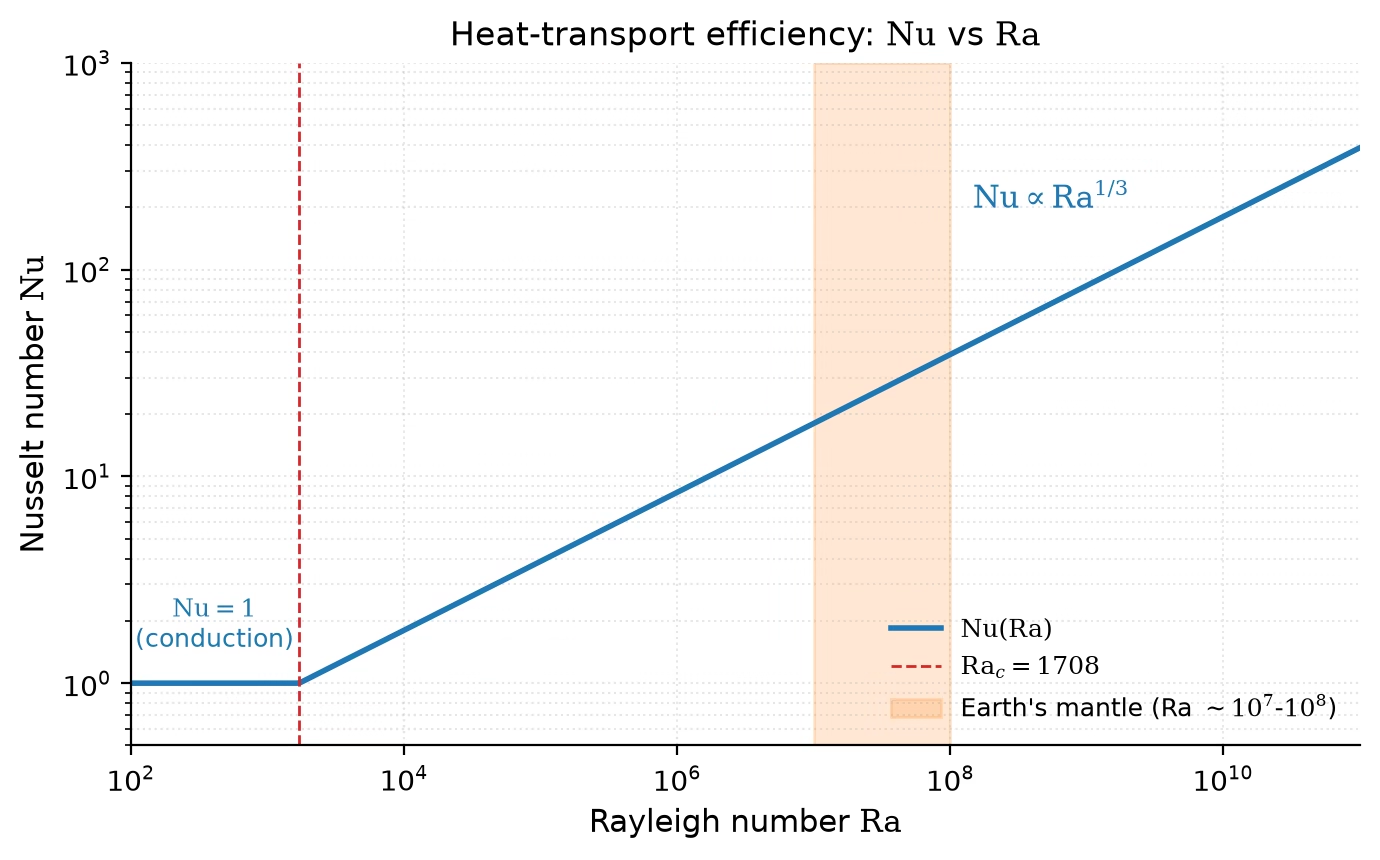
Fig. 8.16 Heat transport efficiency against the Rayleigh number: below \(\mathrm{Ra}_c \approx 1708\) heat is conducted only (\(\mathrm{Nu} = 1\)), above it the boundary-layer scaling \(\mathrm{Nu} \propto \mathrm{Ra}^{1/3}\) applies. Earth’s mantle at \(\eta = 10^{21}\) to \(10^{22}\) Pa s has \(\mathrm{Ra} \sim 10^7\) to \(10^8\) (shaded band), four to five orders of magnitude above the threshold, and transports heat about 20 to 40 times faster than conduction alone under this isoviscous scaling. Course-original figure, first shown in Lecture 3 (Fig. 3.13).

8.6. Phase transitions

As pressure and temperature increase with depth, minerals undergo phase transitions, i.e. rearrangements of their crystal structure to denser configurations. These transitions produce the seismic discontinuities that define the boundaries within Earth’s mantle [Turcotte and Schubert, 2002]:

Depth (km)	Transition	Density change
410	Olivine → wadsleyite	\(\sim\)5% increase
520	Wadsleyite → ringwoodite	\(\sim\)2% increase
660	Ringwoodite → bridgmanite + ferropericlase	\(\sim\)8% increase
\(\sim\)2700	Bridgmanite → post-perovskite	\(\sim\)1–2% increase

The 410 km discontinuity marks the transition of olivine (\(\mathrm{(Mg,Fe)_2SiO_4}\)) to wadsleyite, a denser crystal structure with the same chemical composition. At 660 km, the most dramatic transformation occurs: ringwoodite (the highest-pressure olivine polymorph) breaks down into bridgmanite (\(\mathrm{(Mg,Fe)SiO_3}\), a perovskite-structured phase, a dense mineral structure common at high pressure) plus ferropericlase (\(\mathrm{(Mg,Fe)O}\)). This 660 km discontinuity is the most important internal boundary within the mantle, marking the transition from upper to lower mantle. Its negative Clapeyron slope (the boundary pressure decreases with increasing temperature) means it partially resists the passage of convecting material, influencing the style of mantle convection.

Near the base of the mantle (\(\sim\)2700 km depth), bridgmanite transforms to post-perovskite, a phase discovered in laboratory experiments in 2004 [Murakami et al., 2004]. This transition may explain the seismically anomalous D” layer just above the core-mantle boundary, where seismic velocities show complex lateral variations. Fig. 8.17 summarises the principal phase boundaries against an approximate Earth geotherm.

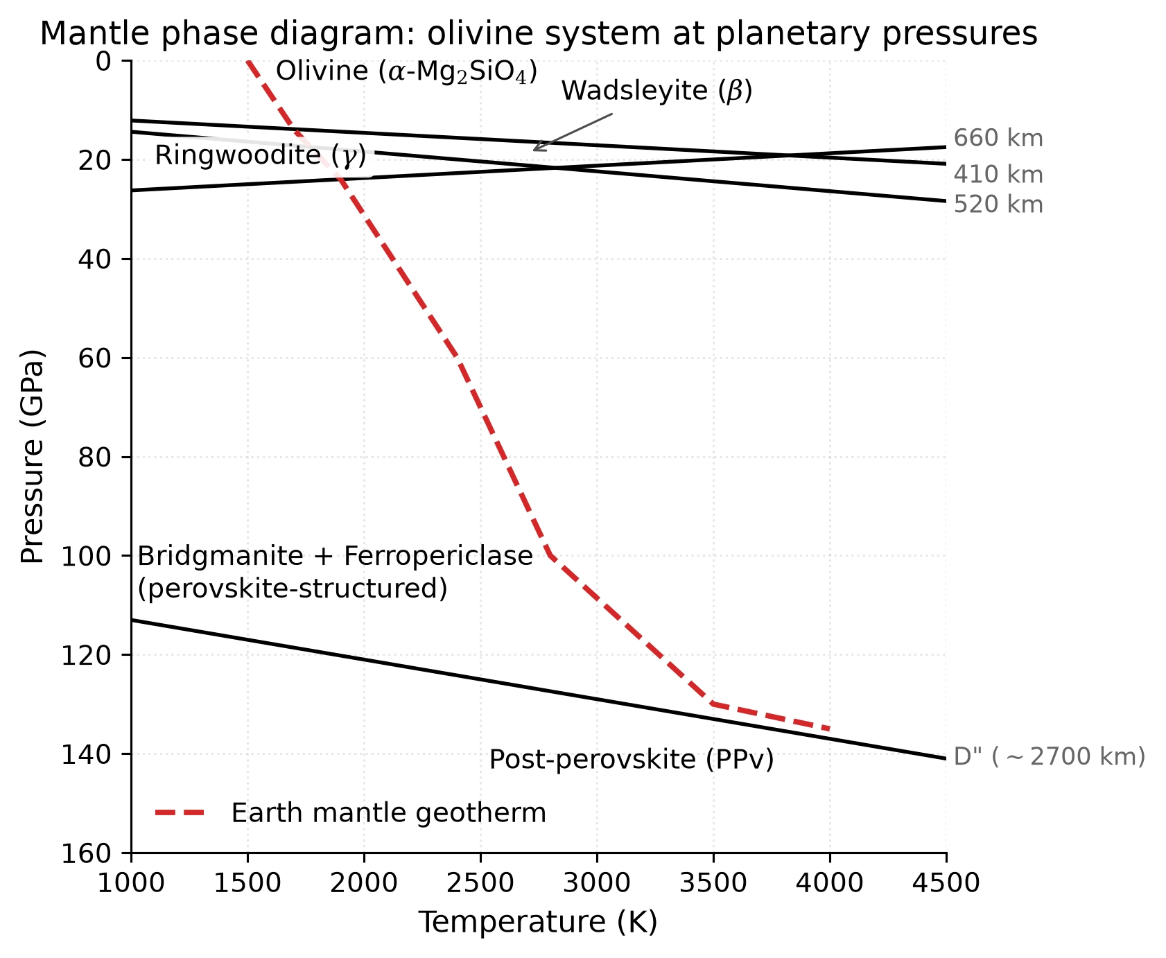
Fig. 8.17 Schematic pressure-temperature phase diagram of the Earth’s mantle in the olivine-bearing system. Solid black lines show the major phase boundaries: olivine (\(\alpha\)-Mg\(_2\)SiO\(_4\)) → wadsleyite (\(\beta\)) at \(\sim\)14 GPa (410 km), wadsleyite → ringwoodite (\(\gamma\)) at \(\sim\)18 GPa (520 km), ringwoodite → bridgmanite + ferropericlase at \(\sim\)24 GPa (660 km), and bridgmanite → post-perovskite (PPv) at \(\sim\)125 GPa (D” layer, \(\sim\)2700 km). The dashed red curve traces an approximate Earth mantle geotherm. The 660 km transition has a negative Clapeyron slope, which partially resists upwelling (rising) and downwelling (sinking) convective material flux. Boundary positions adapted from Turcotte and Schubert [2002] and post-perovskite from laboratory experiments by Murakami et al. [2004]. Schematic; absolute slopes are approximate. Course-original figure.

These phase transitions are not unique to Earth. Any sufficiently large rocky body will experience them at appropriate pressures, though the specific depths depend on the body’s size, gravity, and thermal state. Mars, for example, likely has an olivine-to-wadsleyite transition in its deep mantle, while the Moon is too small to reach the required pressures.

8.7. Comparative terrestrial interiors

While Earth’s interior is uniquely well characterised, we can apply the same principles to other terrestrial bodies (Fig. 8.18). The combination of mean density, \(C/MR^2\), and (where available) seismic data constrains their internal structures [de Pater and Lissauer, 2010].

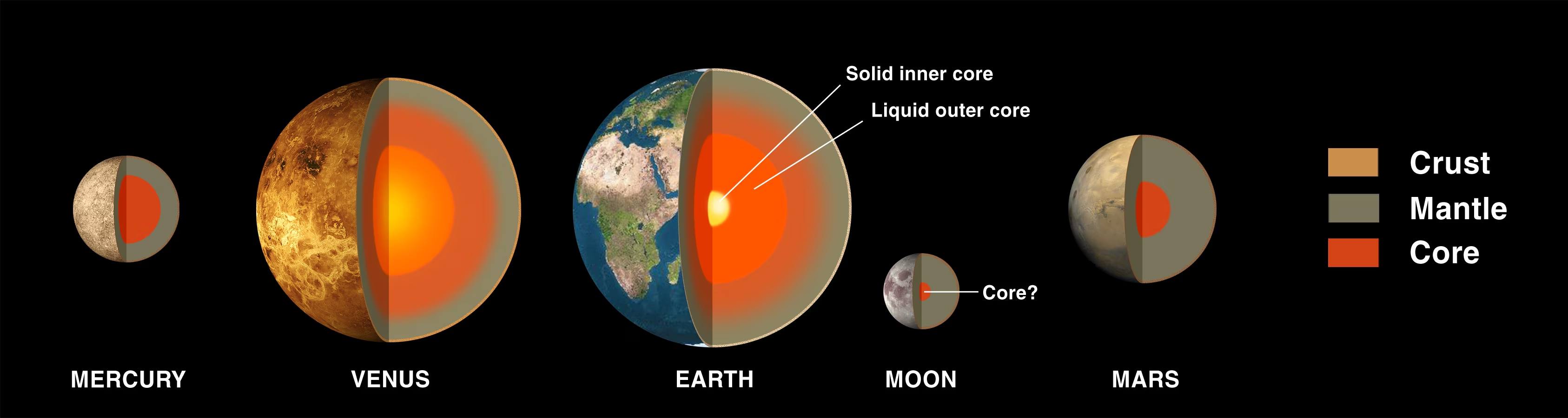
Fig. 8.18 Cross-sections of the four terrestrial planets and Earth’s Moon, drawn to relative size. Crust (orange), silicate mantle (grey), and metallic core (red) are coloured uniformly across the bodies; Earth’s two-component core (solid inner / liquid outer) is shown explicitly. Mercury’s core occupies \(\sim\)83% of its radius and \(\sim\)74% of its mass, the largest core fraction of any terrestrial planet, while the Moon has only a small (\(\sim\)330 km radius) partially molten core. Credit: NASA Solar System Exploration, public domain.

The Moon (\(C/MR^2 = 0.393\), \(\bar{\rho} = 3346\) kg m\(^{-3}\)) is only weakly differentiated. Apollo seismometers (1969–1977), reanalysed with modern processing techniques, revealed a crust \(\sim\)34–43 km thick, a silicate mantle extending to \(\sim\)1400 km depth, and a small partially molten core with radius \(\sim\)200–380 km (only \(\sim\)10–20% of the Moon’s radius: the lower bound from GRAIL and lunar laser ranging gravity inversions [Williams et al., 2014], the upper bound from Apollo seismic reanalysis [Weber et al., 2011]; Fig. 8.19). The near-undifferentiated state (\(C/MR^2\) close to 0.4) and low mean density are consistent with a body that formed primarily from silicate mantle material, supporting the giant impact hypothesis for the Moon’s origin Lecture 2.

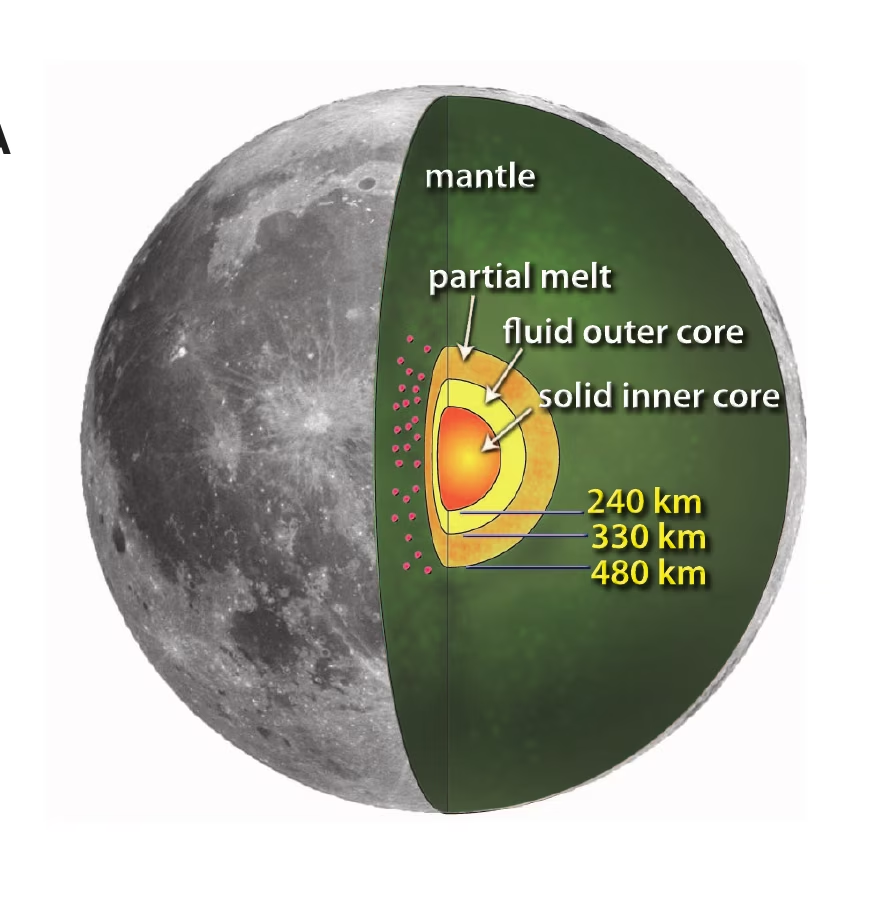
Fig. 8.19 Inferred lunar interior from re-analysis of the Apollo passive seismic experiment, showing a silicate mantle, a partial-melt boundary layer at \(\sim\)480 km from the centre, a liquid Fe-alloy outer core at \(\sim\)330 km radius, and a small solid inner core at \(\sim\)240 km radius. The red dots inside the wedge mark the deep-moonquake source regions used to constrain the deepest part of the interior. The GRAIL+LLR moment of inertia of the solid Moon, \(I_s/MR^2 = 0.392728 \pm 0.000012\) [Williams et al., 2014], is consistent with this layered structure. Reproduced from [Weber et al., 2011], Fig. 1A.

Mars (\(C/MR^2 = 0.364\), \(\bar{\rho} = 3934\) kg m\(^{-3}\)) was transformed from a one-data-point problem into a seismically characterised planet by NASA’s InSight mission [Banerdt et al., 2020] (2018–2022). The SEIS seismometer detected hundreds of marsquakes, revealing a layered internal structure [Khan et al., 2021, Stähler et al., 2021]:

• A crust 24–72 km thick (varying between the thin northern lowlands and thick southern highlands) [Knapmeyer-Endrun et al., 2021]

• A mantle extending to \(\sim\)1560 km depth (i.e. to the top of the core)

• A liquid core of radius \(\sim\)1830 km (\(\sim\)54% of Mars’s radius; later revised downward, see below), composed of iron alloyed with sulfur and other light elements

Fig. 8.20 summarises the structure InSight resolved.

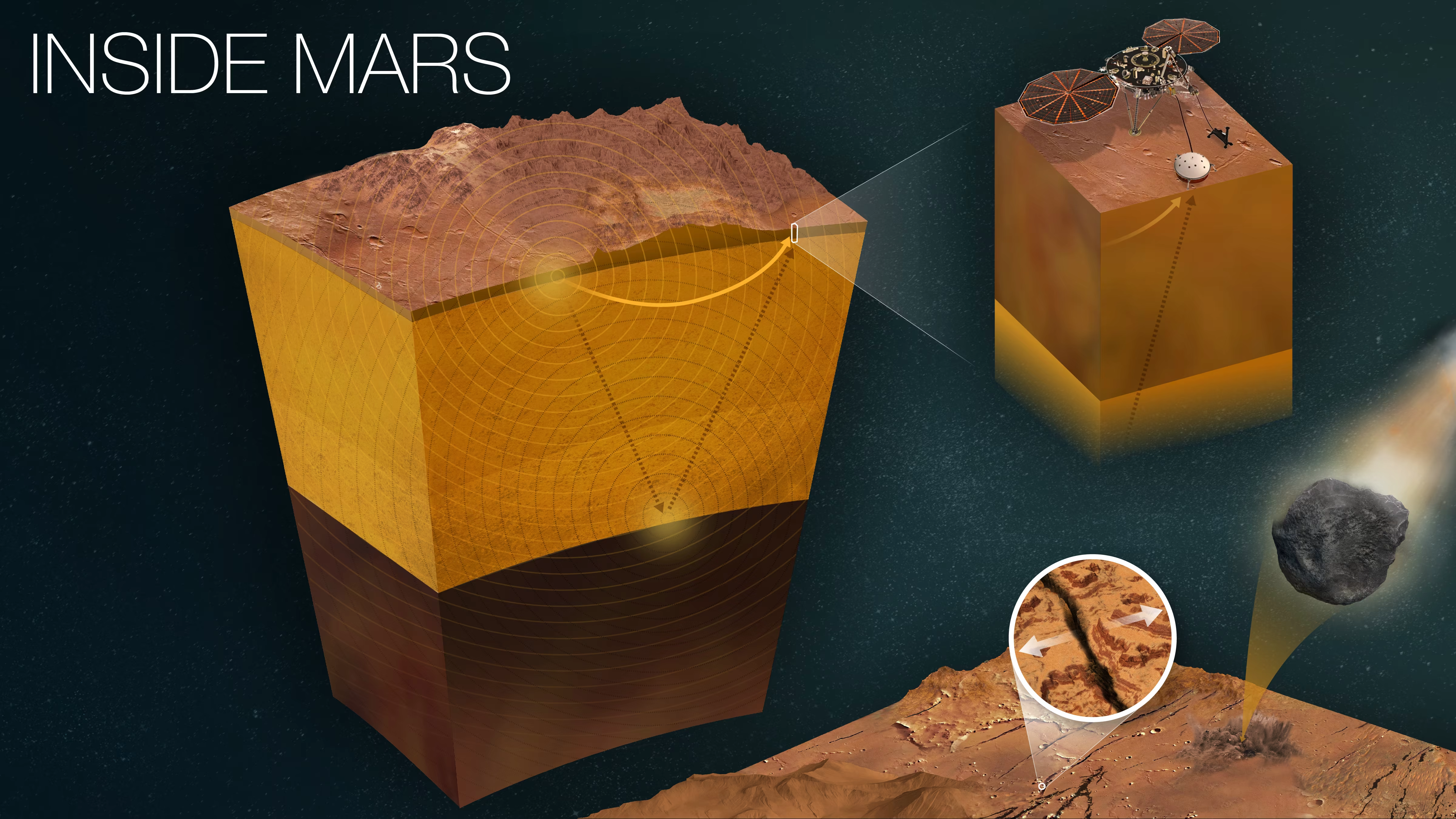
Fig. 8.20 NASA’s “Inside Mars” infographic summarising the interior structure constrained by the InSight mission. The central cutaway block exposes the layered crust, mantle, and liquid Fe-S core (radius \(\sim\)1830 km, \(\sim\)54% of Mars’s radius; later revised downward, see main text). The inset at upper right shows the InSight lander with its SEIS seismometer on the Martian surface; the inset at lower right shows a meteoroid impact and a close-up of the Cerberus Fossae graben region near where many of the largest marsquakes originated. Both impacts and tectonic marsquakes acted as the seismic sources whose travel times revealed the interior layering. Adapted from NASA’s “Inside Mars” infographic, based on results published in [Khan et al., 2021, Stähler et al., 2021]. Credit: NASA/JPL-Caltech (PIA25282).

Mars’s core occupies a comparable fraction of the planet’s radius (54%) to Earth’s outer core (55%), but is far less dense (\(\sim\)6000 kg m\(^{-3}\) vs \(\sim\)10,900 kg m\(^{-3}\)), indicating a higher fraction of light elements, particularly sulfur. The seismic velocity profiles (Fig. 8.21) directly capture this contrast: \(v_S\) drops to zero across the core-mantle boundary, while \(v_P\) steps down because the liquid Fe-S alloy has a smaller bulk modulus than the overlying silicate mantle. Two 2023 reanalyses using marsquakes recorded on the planet’s far side reinterpret the Stähler 2021 boundary as the top of a molten silicate layer (Khan et al. [2023]: \(150 \pm 15\) km thick) rather than the metallic core itself. This revises the iron core radius downward to \(\sim\)1650–1675 km and its density upward to \(\sim\)6470–6650 kg m\(^{-3}\) [Khan et al., 2023, Samuel et al., 2023]. The absence of a present-day global magnetic field suggests the core is no longer convecting vigorously enough to sustain a dynamo, although remnant crustal magnetisation records an ancient field Lecture 4.

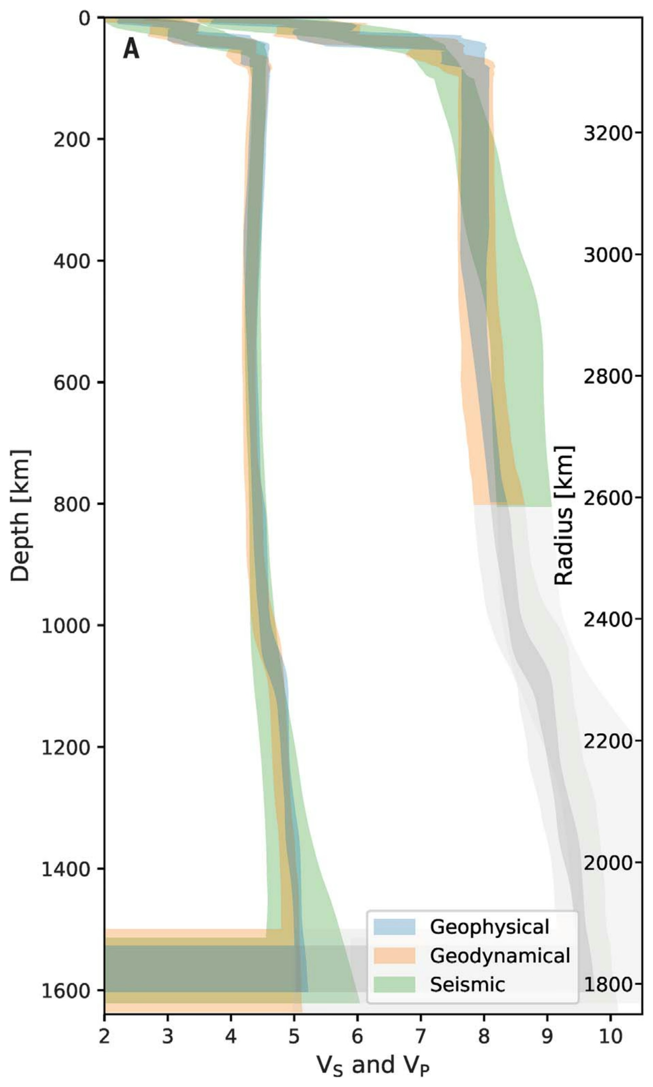
Fig. 8.21 Radial profiles of Mars compressional (\(v_P\)) and shear (\(v_S\)) wave speeds versus depth from three independent InSight inversion approaches: geophysical (blue), geodynamical (orange), and seismic (green). Shaded bands are 95% credible intervals. Below \(\sim\)800 km depth the \(v_P\) profiles enter a region (pale grey shading on the right side of the panel) where direct seismic constraint is no longer available, and the model curves there are extrapolations rather than data-driven inversions; \(v_S\) vanishes at the core-mantle boundary because shear waves do not propagate through the liquid Fe-S outer core. Reproduced from [Stähler et al., 2021], Fig. 2A.

Mercury (\(C/MR^2 = 0.346\), \(\bar{\rho} = 5427\) kg m\(^{-3}\)) presents a puzzle: it has the highest uncompressed density of any terrestrial planet (the density its material would have at zero pressure, correcting for self-compression), implying a very large iron core (Fig. 8.22). Earth-based radar observations of Mercury’s forced libration first established that the core is at least partially molten [Margot et al., 2007]. Combined MESSENGER gravity, libration, and topography data constrain the core radius to \(\sim\)2000–2050 km, approximately 83% of the planet’s radius, and containing \(\sim\)74% of its mass [Margot et al., 2018]. A thin silicate mantle (\(\sim\)400 km) and crust (\(\sim\)30–50 km) overlie this enormous core. Mercury retains a weak but global magnetic field, indicating that at least part of its core is still liquid and convecting. Explaining why Mercury has such a large core fraction remains an active area of research; we return to it in Lecture 10.

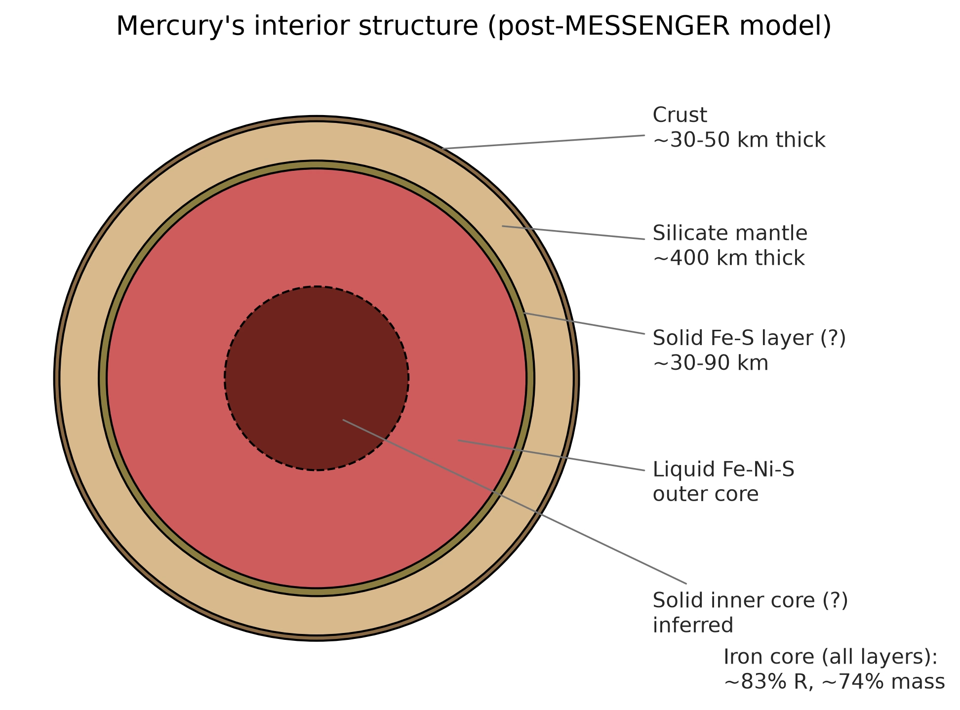
Fig. 8.22 Mercury’s internal structure inferred from MESSENGER gravity and libration data. The crust (\(\sim\)30-50 km) and a thin silicate mantle (\(\sim\)400 km) overlie a large core occupying \(\sim\)83% of Mercury’s radius. The core itself is layered: a possible thin solid Fe-S layer at the top of the core (the “FeS snow zone”), a liquid Fe-Ni-S outer core that sustains the planet’s weak global magnetic field, and an inferred but unresolved solid inner core. The radar libration measurement of Margot et al. [2007] established that the core is at least partially molten; the layer dimensions shown here follow the MESSENGER-era synthesis of Margot et al. [2018]. Course-original figure.

8.8. Giant planet interiors

Jupiter and Saturn are fundamentally different from rocky planets: composed primarily of hydrogen and helium, they lack distinct solid surfaces. Their “surfaces” are conventionally defined as the 1-bar pressure level, and below this the atmosphere transitions continuously into an increasingly dense interior (Fig. 8.23) [Fortney and Nettelmann, 2010].

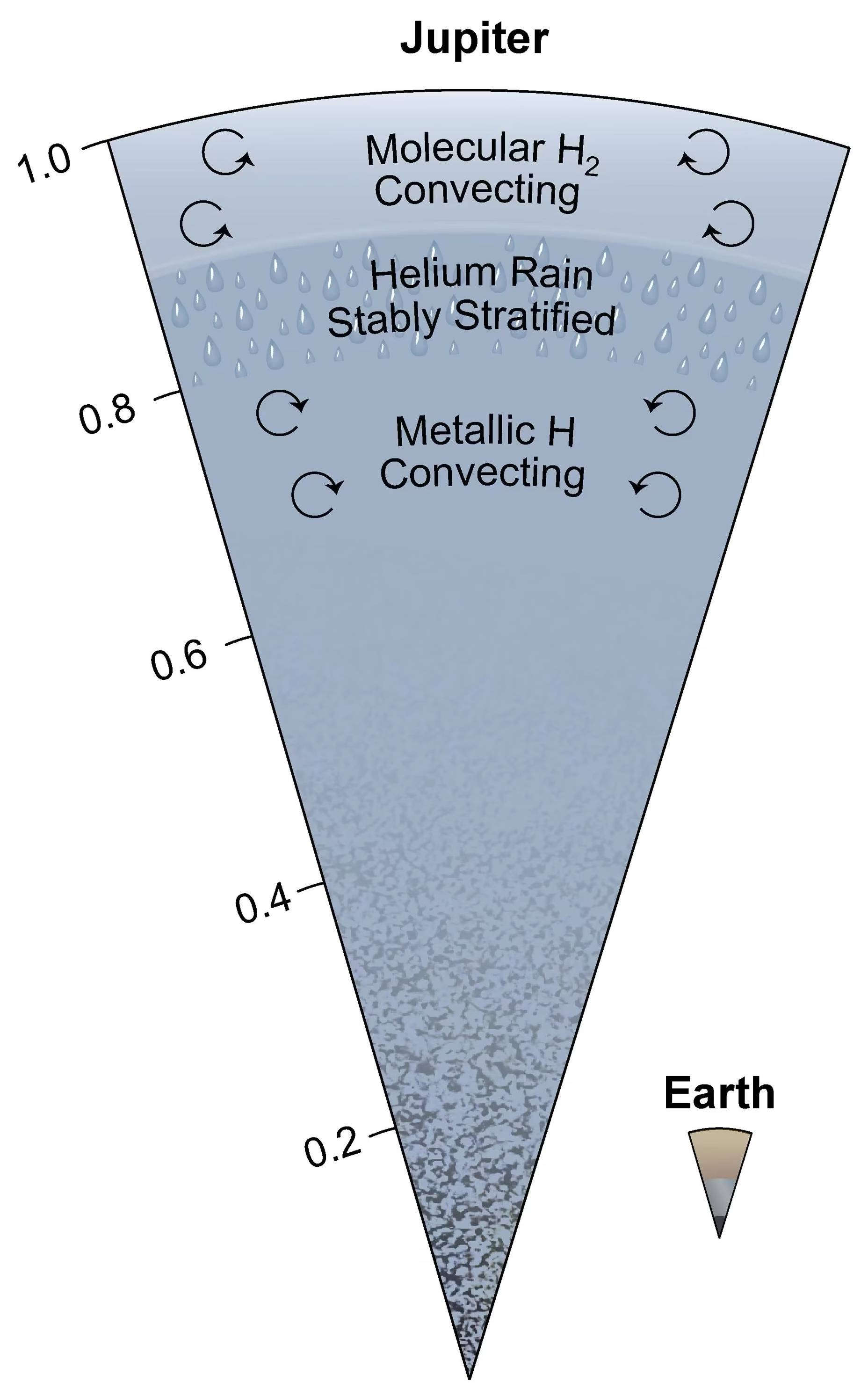
Fig. 8.23 Jupiter’s internal structure shown as a radial cross-section (with Earth for scale at lower right). The outermost layer is convecting molecular \(\mathrm{H_2}\). Below, a helium rain layer forms a stably stratified region where helium droplets settle inward. Deeper still, metallic hydrogen (hydrogen compressed enough that its electrons become delocalised, so it conducts electricity like a metal) convects vigorously, generating Jupiter’s powerful magnetic field. The core region (bottom) shows a gradual increase in heavy-element concentration, the dilute core inferred from Juno gravity data [Wahl et al., 2017]. Credit: NASA/JPL-Caltech/SwRI/John E. Connerney (PIA25062).

Jupiter (\(M = 318\,\Mearth\), \(R = 11.2\,\Rearth\)) has been characterised with unprecedented precision by the Juno mission (2016 to present), which measures Jupiter’s gravity field to high accuracy. The interior can be described in broad terms:

• Molecular hydrogen envelope (outer ~15% by radius): \(\mathrm{H_2}\) gas transitioning to liquid, \(\rho \sim 0.2\)–\(1\) g cm\(^{-3}\)

• Metallic hydrogen layer (extending to ~80% of the radius): at pressures above \(\sim\)1–4 Mbar (\(10^{11}\)–\(4 \times 10^{11}\) Pa), hydrogen undergoes a gradual transition to a metallic state where electrons are delocalised and the material conducts electricity. This conducting metallic hydrogen is the source of Jupiter’s powerful magnetic field (Lecture 4)

• Core region: Juno’s gravity data show that most of the heavy elements (rock and ice) are not concentrated in a small compact core but are instead spread over a large dilute core extending to perhaps 30–50% of Jupiter’s radius (Fig. 8.24) [Wahl et al., 2017]. The dilute core may be a relic of the formation process or the result of erosion of an initially compact core by convective mixing. The competing interior model suites for Jupiter’s dilute core and their implications for giant planet formation are examined in Lecture 11.

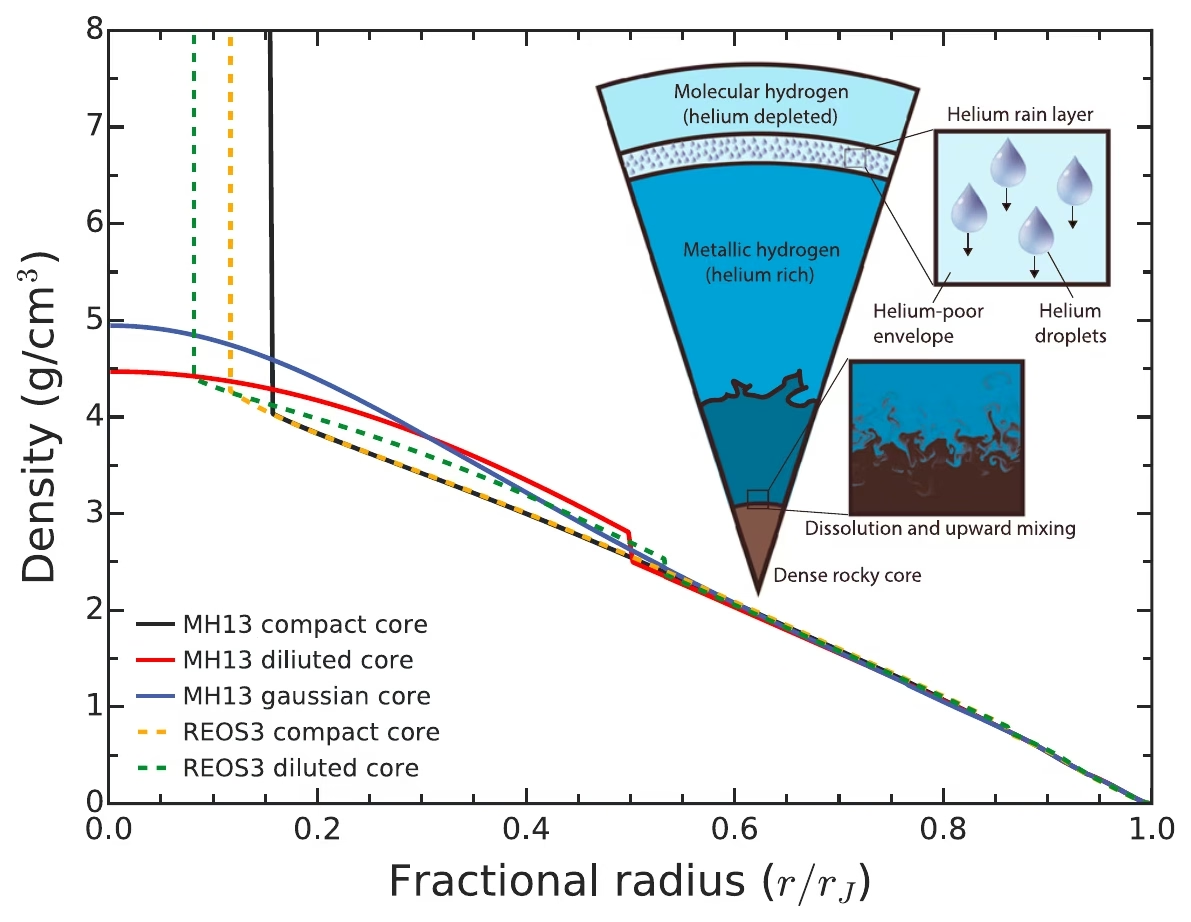
Fig. 8.24 Density profiles of representative Jupiter interior models. Solid curves use the MH13 hydrogen equation of state and dashed curves use REOS3. Black: a compact-core model with constant heavy-element enrichment inside \(r/r_J = 0.15\) matching the Galileo entry-probe envelope composition. Red (Model D): a Juno-fitting model with \(Z = 0.007\) in the molecular envelope and a constant-\(Z\) “dilute” or “fuzzy” core expanded to \(r/r_J \sim 0.5\). Blue (Model E): an alternative dilute-core solution with a Gaussian \(Z\) profile. Orange (Model R) and green (Model S): REOS3-based compact and dilute cores respectively. The schematic cross-section at top right indicates the inferred layered structure for the dilute-core solutions: an outer molecular hydrogen-helium envelope, a helium-rain layer, and a metallic hydrogen region overlying a graded heavy-element core. Reproduced from [Wahl et al., 2017], Fig. 1.

Central conditions reach approximately 4000 GPa and 20,000 K. Jupiter radiates roughly 1.7 times the energy it receives from the Sun, indicating substantial internal heat production from ongoing gravitational contraction (the Kelvin-Helmholtz mechanism).

Saturn (\(M = 95\,\Mearth\), \(R = 9.4\,\Rearth\)) shares Jupiter’s overall structure but with some key differences (Fig. 8.25). Saturn’s lower mass means pressures are lower throughout, so the metallic hydrogen transition occurs deeper. Saturn also has a larger proportional heavy-element enrichment.

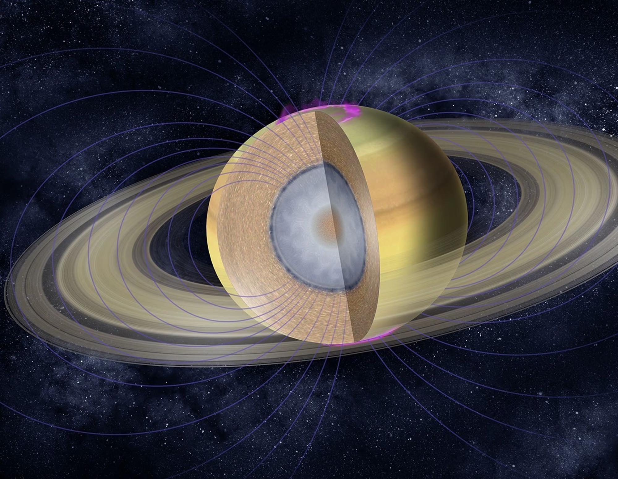
Fig. 8.25 Cutaway artist’s concept of Saturn’s interior, with rings, magnetic field lines, and aurorae. The rendering shows the molecular hydrogen envelope (brown), a metallic hydrogen layer (grey) where the magnetic dynamo operates, and a central heavy-element core (orange/white). The diffuse-core inference from Mankovich and Fuller [2021] modifies the classical sharp-core picture: heavy elements are gradationally distributed over the inner \(\sim\)60% of the planet’s radius. Credit: NASA/JPL-Caltech.

A notable process in Saturn’s interior is helium rain: as the planet cools, helium becomes immiscible in metallic hydrogen at \(P \approx 2\) Mbar and forms droplets that settle toward the centre, releasing gravitational energy and explaining Saturn’s unexpectedly high heat output (Fig. 8.26) [Mankovich and Fortney, 2020]. Saturn radiates about 1.8 times the absorbed solar flux, more than expected from simple contraction alone. Ring seismology with Cassini data shows that Saturn, like Jupiter, has a diffuse heavy-element core [Mankovich and Fuller, 2021]; Lecture 11 takes up that result.

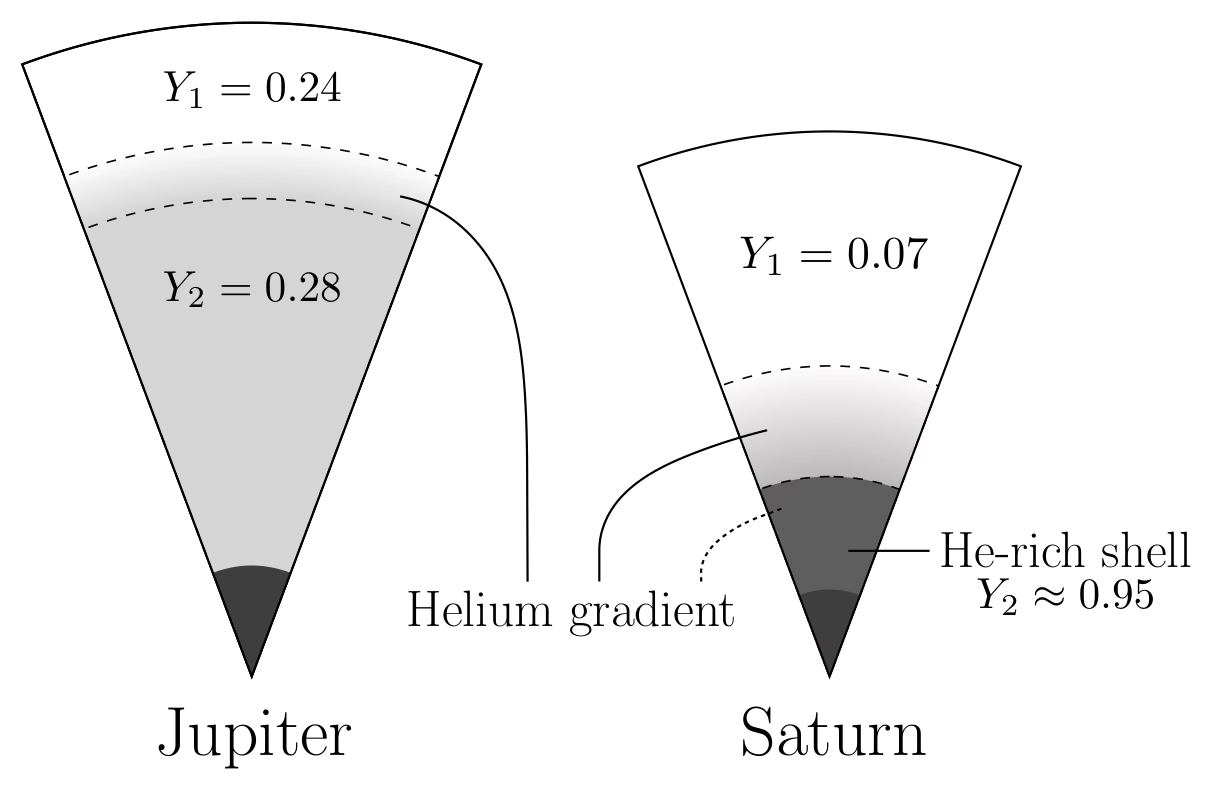
Fig. 8.26 Comparative schematic of Jupiter and Saturn showing where helium phase separation deposits a continuous helium-gradient region (between the dashed boundaries) on top of the deep envelope. In Jupiter, the favoured solution is a thin gradient extending from the onset of hydrogen-helium immiscibility at \(P \approx 2\) Mbar (outer dashed line at \(\approx 80\%\) of the planet’s radius) to a deeper envelope with helium mass fraction \(Y_2 = 0.28\). In Saturn, the gradient is more extensive, reaching from \(P \approx 2\) Mbar (outer dashed line at \(\approx 55\%\) of the radius) down to a helium-rich shell with \(Y_2 \approx 0.95\) at \(\approx 35\%\) of the radius. Wedges are scaled to each planet’s radius. Reproduced from [Mankovich and Fortney, 2020], Fig. 3.

8.9. Ice giant interiors

Uranus (\(M = 14.5\,\Mearth\)) and Neptune (\(M = 17.1\,\Mearth\)) are often called ice giants to distinguish them from the gas giants, because a large fraction of their mass consists of heavier molecules (primarily water (\(\mathrm{H_2O}\)), ammonia (\(\mathrm{NH_3}\)), and methane (\(\mathrm{CH_4}\))) rather than hydrogen and helium [Fortney and Nettelmann, 2010].

The canonical three-layer model consists of:

1. Hydrogen-helium envelope (outermost \(\sim\)20% by mass): molecular gas transitioning to denser fluid

2. Ice/fluid layer (\(\sim\)60–70% by mass): a hot, dense fluid of water, ammonia, and methane at pressures of \(\sim\)10–500 GPa and temperatures of \(\sim\)2000–7000 K. Despite the name “ice,” this material is a hot ionic fluid; in part of the layer it may transition into a predicted superionic state, in which oxygen atoms form a crystalline lattice while hydrogen ions diffuse freely and the material conducts electricity, although the existence and depth range of this phase inside Uranus and Neptune remain uncertain

3. Rocky core (\(\sim\)10–20% by mass): silicates and iron at the centre, though the boundary with the ice layer may be gradational (Fig. 8.27); whether the layers are distinct or graded is an open question taken up in Lecture 11

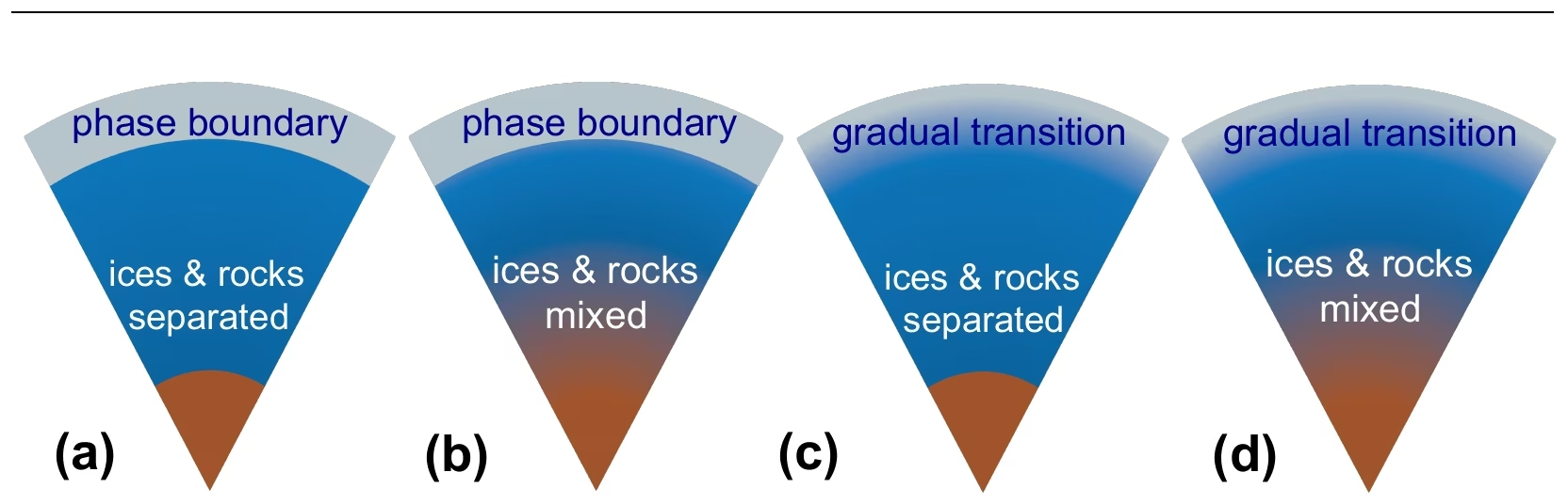
Fig. 8.27 Sketches of four possible internal structures of an ice giant (Uranus or Neptune). It is unclear whether the planets are differentiated and whether the transition between layers is distinct or gradual: (a) sharp phase boundary between the H-He envelope and the icy layer, with ices and rocks separated; (b) sharp phase boundary at the H-He/ice interface, ices and rocks mixed below; (c) gradual transition between the H-He envelope and the ice layer, with a sharp boundary between ice and rock; (d) gradual transitions both at the H-He/ice and ice/rock interfaces, suggesting a global composition gradient. Reproduced from [Helled et al., 2020], Fig. 4.

The magnetic fields of Uranus and Neptune are strikingly unusual: both are strongly tilted relative to the rotation axis (59° for Uranus, 47° for Neptune) and offset from the planet’s centre. This contrasts sharply with the roughly dipolar, axially aligned fields of Earth, Jupiter, and Saturn (Fig. 8.28). The explanation likely involves the geometry of the conducting region: rather than being generated in a deep metallic hydrogen shell (as in Jupiter), the ice giant dynamos may operate in the shallow, thin conducting ice layer, producing more complex field geometries.

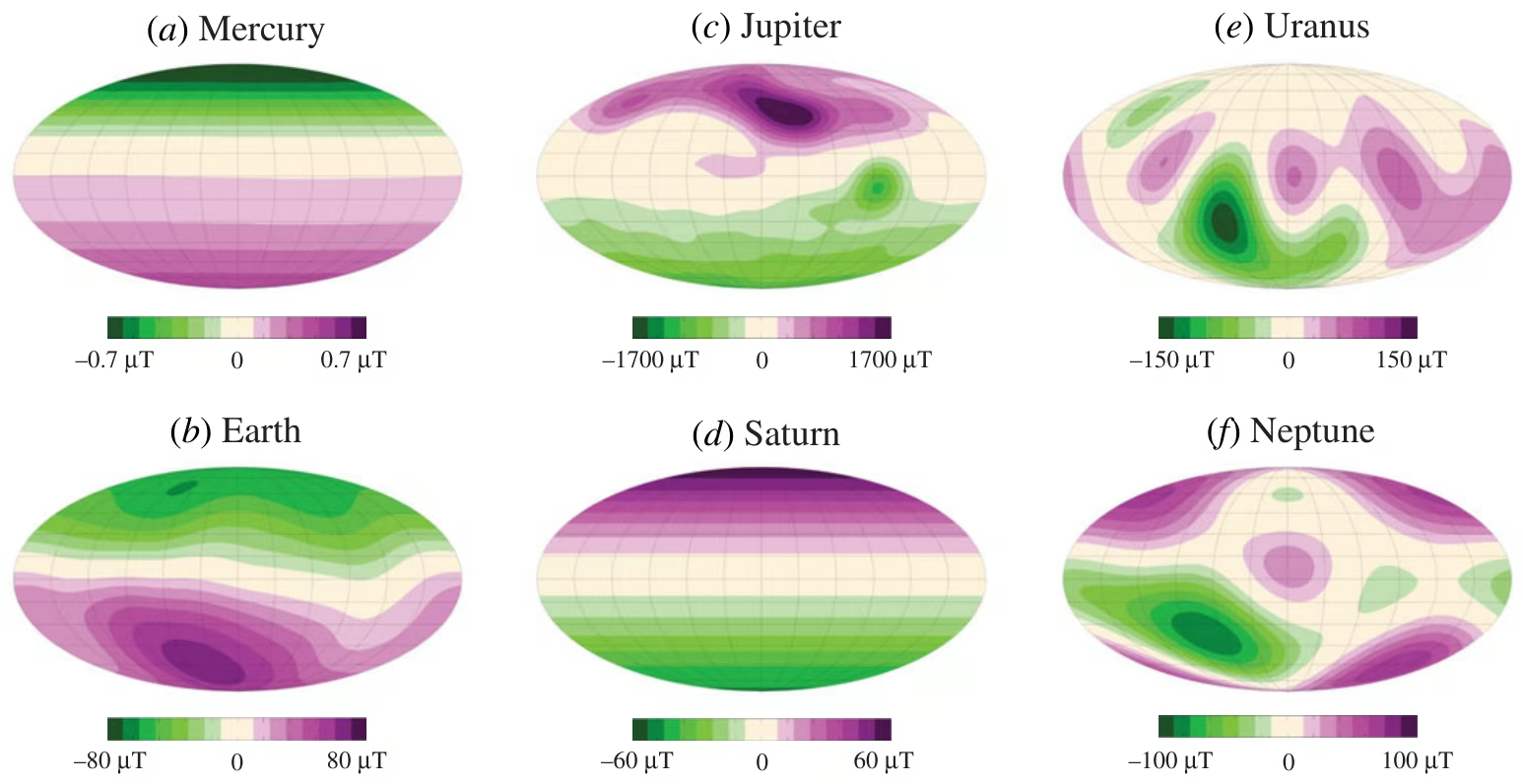
Fig. 8.28 Radial magnetic field at the surface of (a) Mercury, (b) Earth, (c) Jupiter, (d) Saturn, (e) Uranus and (f) Neptune in Mollweide projection, each panel with its own colour scale. Earth, Jupiter and Saturn carry dipoles nearly aligned with the rotation axis; the Uranus and Neptune fields are multipolar, tilted by \(\sim 59^\circ\) and \(\sim 47^\circ\) and offset from the centre; Mercury’s weak field has its dipole shifted \(\sim 500\) km north. Reproduced from [Soderlund and Stanley, 2020], Fig. 1; Lecture 4 discusses the dynamos behind them.

Neptune emits \(\sim\)2.6 times the solar energy it absorbs, while Uranus has essentially no measurable internal heat excess, a long-standing puzzle. Proposed explanations include compositional gradients that inhibit convection in Uranus’s interior, trapping heat within, while Neptune convects more freely. This remains one of the key open questions motivating future ice giant missions, and we examine it further in Lecture 11.

8.10. Icy moon interiors

Among the most remarkable discoveries in planetary science is that several moons in the outer solar system harbour subsurface liquid water oceans beneath their icy shells (Fig. 8.29). These ocean worlds are prime targets for astrobiology because they provide the three key ingredients for life: liquid water, chemical energy, and organic molecules (Lecture 7; Lecture 14 develops the astrobiological case) [Nimmo and Pappalardo, 2016].

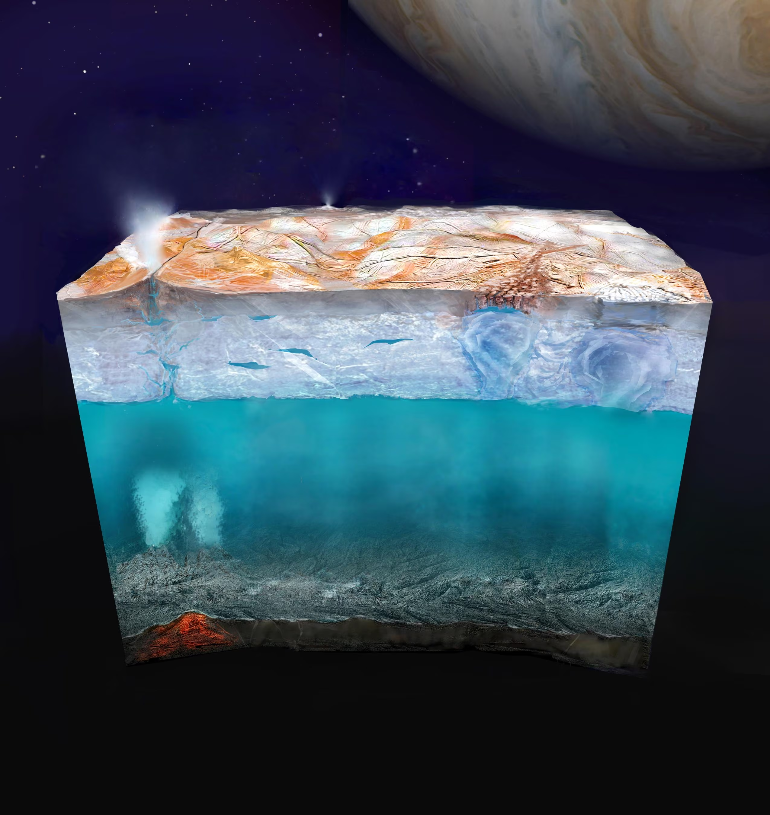
Fig. 8.29 Artist’s concept of Europa’s subsurface environment. The cross-section reveals (top to bottom): the fractured ice surface with plume activity, the ice shell with possible convective features, the global liquid water ocean, and the rocky seafloor where hydrothermal vents may provide chemical energy for life. Jupiter looms in the background. The ocean is estimated to be roughly 100 km deep. Credit: NASA/JPL-Caltech (PIA26438).

Europa (\(R = 1561\) km, \(\rho = 3013\) kg m\(^{-3}\)) has an ice shell estimated at a few to a few tens of kilometres thick, overlying a global ocean roughly 100 km deep [Nimmo and Pappalardo, 2016]. The evidence comes from multiple sources: magnetic induction measurements by the Galileo spacecraft (a time-varying magnetic field induced by Jupiter’s rotating magnetosphere, requiring a near-surface conducting layer), surface geology (disrupted ice blocks in chaos terrain that resemble terrestrial sea ice), and gravity data. Tidal heating (frictional heating generated as a moon’s interior flexes under a planet’s changing gravitational pull along an eccentric orbit) from Europa’s orbital eccentricity, maintained by the Laplace resonance with Io and Ganymede (Fig. 8.30), provides the energy to keep the ocean liquid. Europa Clipper and JUICE, both on their way to the Jupiter system, return in Lecture 11.

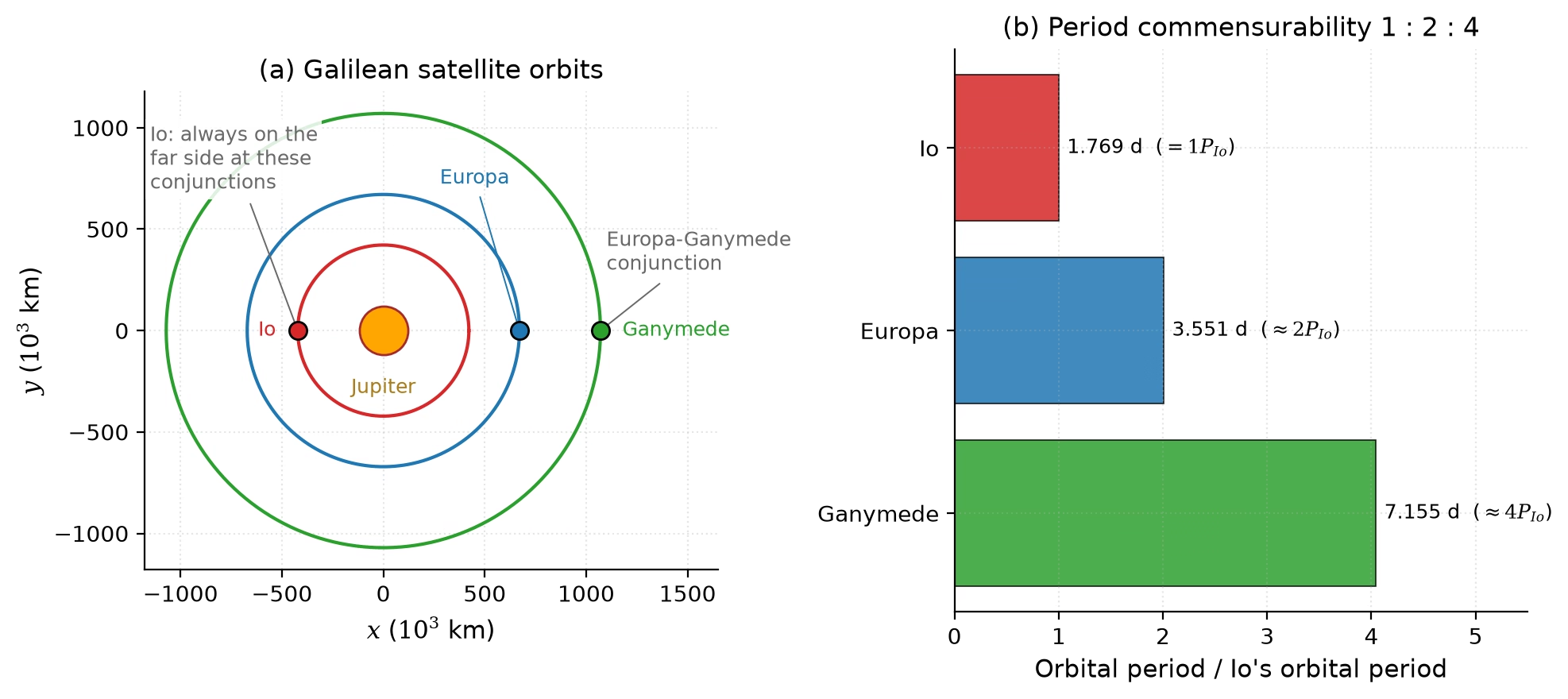
Fig. 8.30 The Io-Europa-Ganymede Laplace resonance that powers Europa’s ocean: (a) the three orbits at a Europa-Ganymede conjunction, (b) the orbital periods in the ratio 1:2:4, so the mean motions stand in the ratio \(n_{\rm Io} : n_{\rm Eur} : n_{\rm Gan} = 4 : 2 : 1\). Repeated conjunctions force small but non-zero orbital eccentricities against tidal damping, producing the time-varying tidal flexing that heats Europa’s interior and maintains its subsurface ocean [Hussmann et al., 2006]. Course-original figure, first shown in Lecture 3 (Fig. 3.27).

Enceladus (\(R = 252\) km, \(\rho = 1609\) kg m\(^{-3}\)) provides the most direct evidence for a subsurface ocean: the Cassini spacecraft flew through geysers of water vapour and ice particles erupting from four fractures (the “tiger stripes”) near the south pole [Porco et al., 2006] (see also Lecture 7). Enceladus’s subsurface ocean is inferred to be global from libration measurements despite the moon’s small size (Fig. 8.31), maintained liquid by tidal heating sustained through the orbital resonance with Dione; the south-polar terrain radiates \(\sim\)15.8 GW [Howett et al., 2011], far more than radiogenic heating can supply, with plume geochemistry and hydrothermal activity explored in Lecture 11.

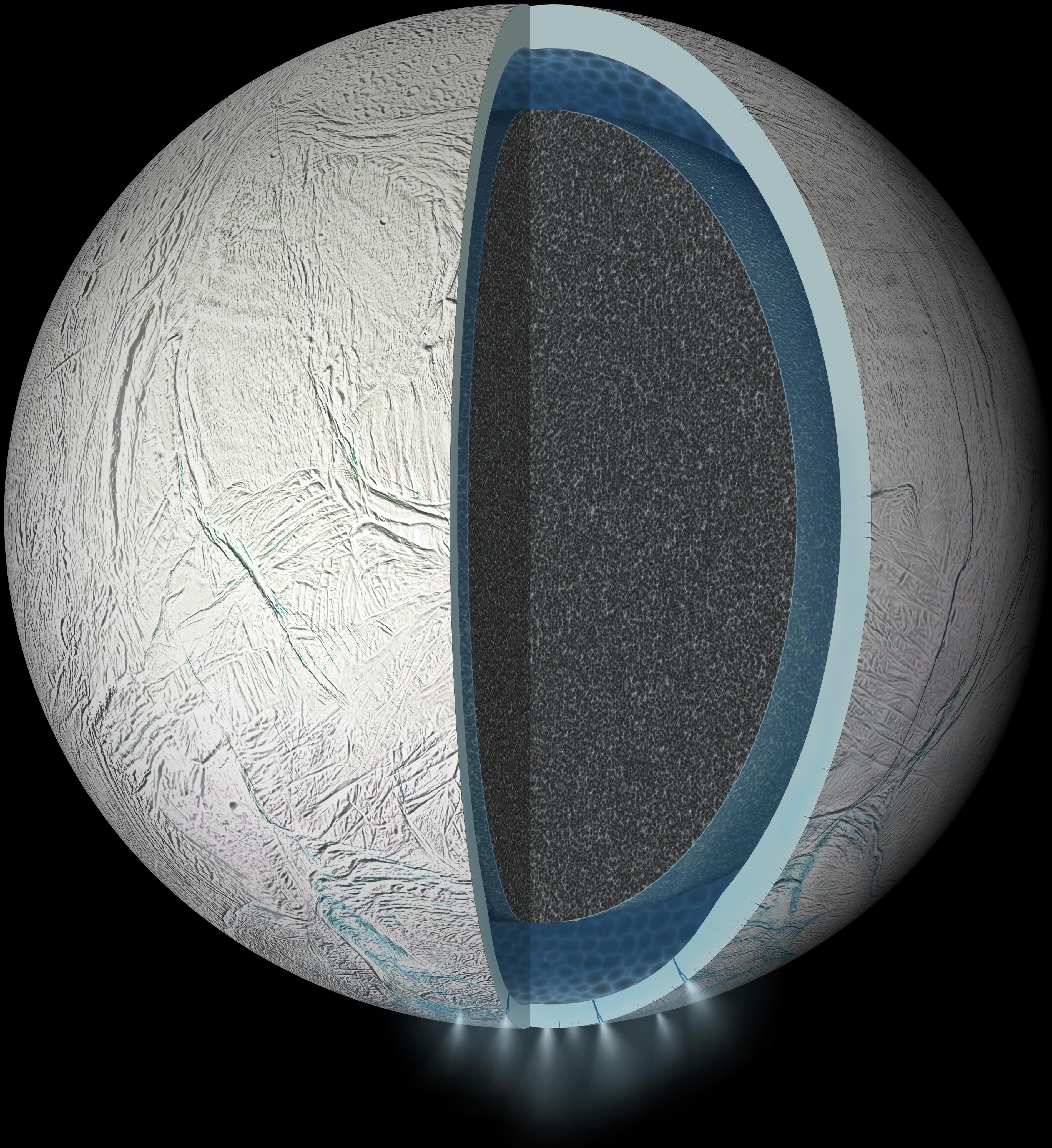
Fig. 8.31 Cutaway artist’s rendering of Enceladus’s interior with a global subsurface liquid water ocean (blue) sandwiched between an icy crust (light grey) and a porous rocky core (dark grey). Active venting from the south polar terrain was first reported by Porco et al. [2006]; the global geometry of the ocean was subsequently inferred from libration measurements of the moon’s small physical librations. The plume sources at the south polar terrain are visible at the bottom. Credit: NASA/JPL-Caltech (PIA19656).

Titan (\(R = 2575\) km, \(\rho = 1882\) kg m\(^{-3}\)) likely harbours a subsurface water-ammonia ocean beneath a thick ice shell (\(\sim\)50–100 km): Cassini’s Doppler tracking measured a tidal Love number \(k_2\) too large for a rigid body, which implies a global ocean that decouples the shell from the rocky interior (Fig. 8.32) [Iess et al., 2012, Sotin et al., 2021]. Titan’s surface, its methane cycle and the Dragonfly mission return in Lecture 11.

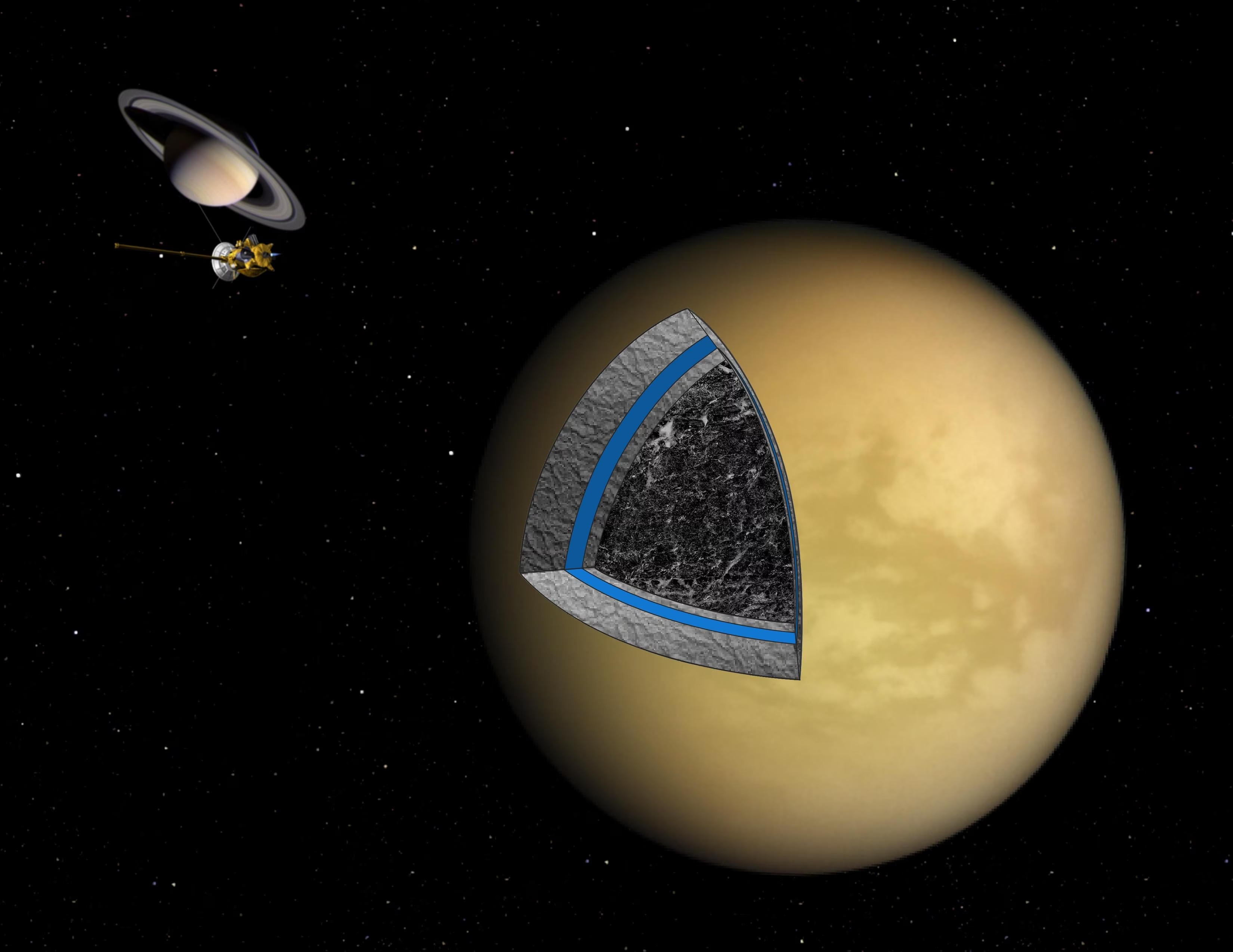
Fig. 8.32 Cutaway artist’s concept of Titan’s interior based on Cassini gravity and radio-science data. The cross-section shows (outer to inner) a methane-bearing atmosphere, an outer ice shell (\(\sim\)50–100 km thick, light grey), a subsurface water-ammonia ocean (blue band), an inner high-pressure ice layer (light grey), and a partially differentiated mix of rock and ice in the deep interior (dark grey). The Cassini-Huygens spacecraft at upper left is not to scale. Credit: NASA/JPL.

The existence of these ocean worlds demonstrates that the classical habitable zone (defined by the distance from a star where liquid water can exist on a surface) is far too narrow a concept. Tidal heating, radiogenic heating (Lecture 3), and insulating ice shells can maintain liquid water far beyond the snow line, vastly expanding the potential environments for life in the universe.

8.11. Recent advances

NASA’s InSight mission (2018–2022) turned Mars from a one-number problem into a seismically characterised planet. Its SEIS instrument recorded marsquakes, and shear waves reflected off the core from near-side events revealed a liquid iron-alloy core [Stähler et al., 2021], below a mantle that ends at \(\sim\)1560 km depth and a crust 24–72 km thick [Knapmeyer-Endrun et al., 2021] (Fig. 8.33). Far-side quakes and meteoroid impacts recorded from late 2021 gave waves that crossed the core, and the 2023 reanalyses of them place a molten silicate layer above a smaller core [Khan et al., 2023, Samuel et al., 2023]: one seismometer rewrote the interior twice in two years. These are the first seismological constraints on another planet’s interior since Apollo; Lecture 10 follows the waveforms themselves.

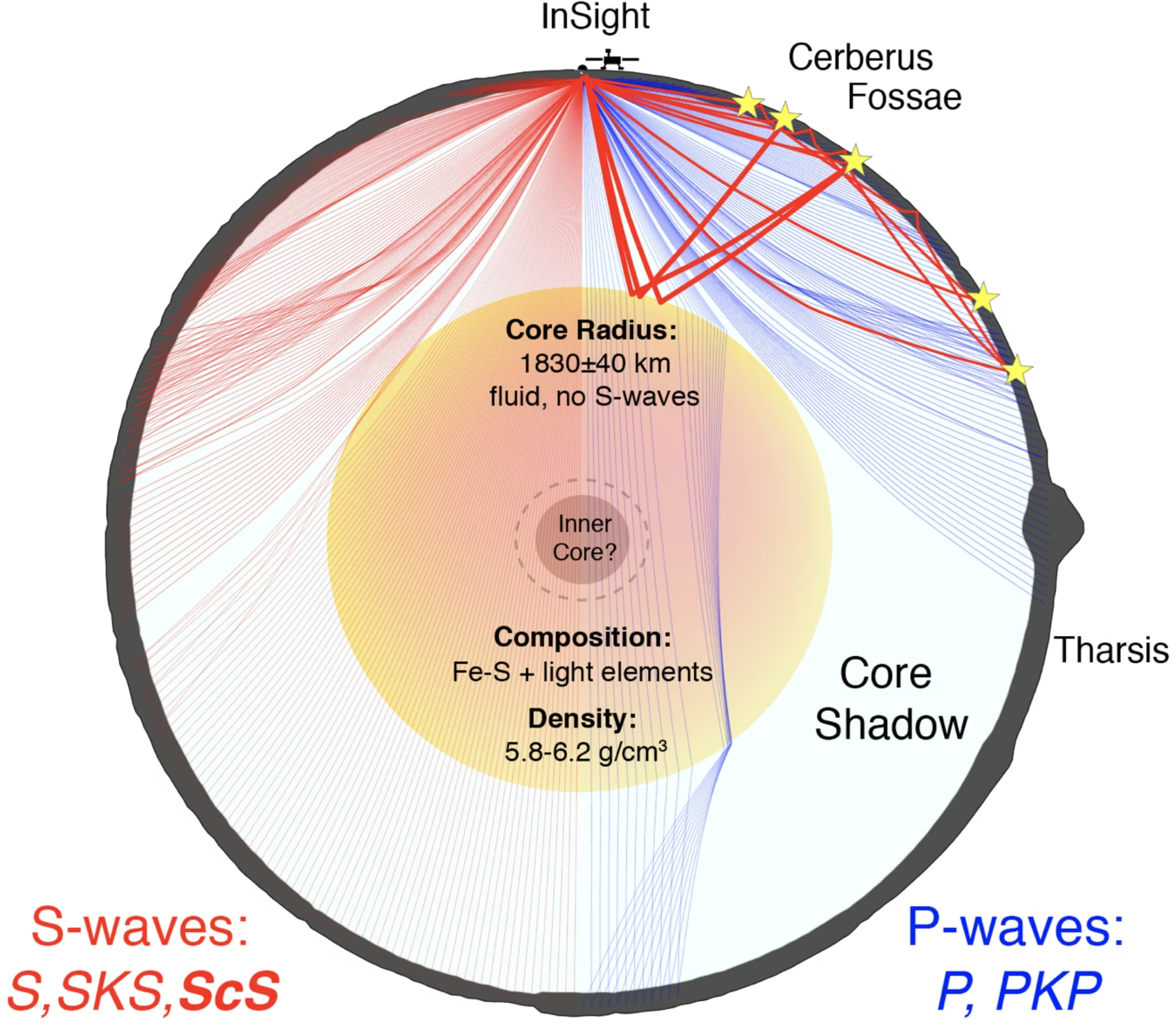
Fig. 8.33 Schematic diagram of Mars’s interior structure inferred from InSight seismology. The cross-section depicts the core-induced shadow zone for seismic waves on a great-circle arc from InSight through Olympus Mons. The S-wave shadow zone is minimal and probably filled by diffracted S-waves (Sdiff), while the P-wave shadow zone is significant and contains specifically the Tharsis region. Annotated values: \(1830 \pm 40\) km seismic-discontinuity radius (interpreted by Stähler et al. [2021] as the core-mantle boundary; \(\rho \approx 5.7\text{-}6.3\) g cm\(^{-3}\) on that interpretation), with no S-waves transmitted below it. The 2023 reanalyses [Khan et al., 2023, Samuel et al., 2023] reinterpret this discontinuity as the top of a molten silicate layer (Khan et al. [2023]: \(150 \pm 15\) km thick) overlying the metallic core, placing the iron-core radius at \(\sim\)1650–1675 km (see preceding text). Reproduced from [Stähler et al., 2021], Fig. 3 (preprint figure numbering; the published Science paper uses the same numbering).

8.12. References

[Aitta2012]

Aitta, A. 2012. “Venus' internal structure, temperature and core composition.” Icarus, 218(2):967–974. doi:10.1016/j.icarus.2012.01.007, https://ui.adsabs.harvard.edu/abs/2012Icar..218..967A/abstract.

[Attia2026] (1,2,3)

Attia, Mara, Lichtenberg, Tim, Jungová, Ema, and Sastre, Mariana. 2026. “PALEOS: multiphase equations of state and mass-radius relations for exoplanet interiors.” Astronomy & Astrophysics. in press. arXiv:2605.03741, https://arxiv.org/abs/2605.03741.

[Banerdt2020]

Banerdt, W. Bruce, Smrekar, Suzanne E., Banfield, Don, Giardini, Domenico, Golombek, Matthew, Johnson, Catherine L., Lognonné, Philippe, Spiga, Aymeric, Spohn, Tilman, Perrin, Clément, Stähler, Simon C., Antonangeli, Daniele, Asmar, Sami, Beghein, Céline, Bowles, Neil, Bozdağ, Ebru, Chi, Peter, Christensen, Ulrich, Clinton, John, Collins, Gareth S., Daubar, Ingrid, Dehant, Véronique, Drilleau, Mélanie, Fillingim, Matthew, Folkner, William, Garcia, Raphaël F., Garvin, James, Grant, John, Grott, Matthias, Grygorczuk, Jerzy, Hudson, Troy, Irving, Jessica C. E., Kargl, Günter, Kawamura, Taichi, Kedar, Sharon, King, Scott, Knapmeyer-Endrun, Brigitte, Knapmeyer, Martin, Lemmon, Mark, Lorenz, Ralph, Maki, Justin N., Margerin, Ludovic, McLennan, Scott M., Michaut, Chloé, Mimoun, David, Mittelholz, Anna, Mocquet, Antoine, Morgan, Paul, Mueller, Nils T., Murdoch, Naomi, Nagihara, Seiichi, Newman, Claire, Nimmo, Francis, Panning, Mark, Pike, W. Thomas, Plesa, Ana-Catalina, Rodriguez, Sébastien, Rodriguez-Manfredi, Jose Antonio, Russell, Christopher T., Schmerr, Nicholas, Siegler, Matthew, Stanley, Sabine, Stutzmann, Eleonore, Teanby, Nicholas, Tromp, Jeroen, van Driel, Martin, Warner, Nicholas, Weber, Renee, and Wieczorek, Mark. 2020. “Initial results from the InSight mission on Mars.” Nature Geoscience, 13(3):183–189. doi:10.1038/s41561-020-0544-y, https://ui.adsabs.harvard.edu/abs/2020NatGe..13..183B/abstract.

[Birch1952] (1,2)

Birch, Francis. 1952. “Elasticity and constitution of the Earth's interior.” Journal of Geophysical Research, 57(2):227–286. doi:10.1029/JZ057i002p00227, https://ui.adsabs.harvard.edu/abs/1952JGR....57..227B/abstract.

[dePaterLissauer2010] (1,2)

de Pater, Imke and Lissauer, Jack J. 2010. Planetary Sciences. Cambridge University Press, Cambridge, 2nd edition. doi:10.1017/cbo9780511780561.

[Dziewonski1981] (1,2,3,4,5,6,7,8)

Dziewonski, Adam M. and Anderson, Don L. 1981. “Preliminary reference Earth model.” Physics of the Earth and Planetary Interiors, 25(4):297–356. doi:10.1016/0031-9201(81)90046-7, https://ui.adsabs.harvard.edu/abs/1981PEPI...25..297D/abstract.

[FortneyNettelmann2010] (1,2)

Fortney, Jonathan J. and Nettelmann, Nadine. 2010. “The interior structure, composition, and evolution of giant planets.” Space Science Reviews, 152(1–4):423–447. doi:10.1007/s11214-009-9582-x, arXiv:0912.0533, https://ui.adsabs.harvard.edu/abs/2010SSRv..152..423F/abstract.

[French2015]

French, Scott W. and Romanowicz, Barbara. 2015. “Broad plumes rooted at the base of the Earth's mantle beneath major hotspots.” Nature, 525(7567):95–99. doi:10.1038/nature14876, https://ui.adsabs.harvard.edu/abs/2015Natur.525...95F/abstract.

[Fukao2013] (1,2)

Fukao, Yoshio and Obayashi, Masayuki. 2013. “Subducted slabs stagnant above, penetrating through, and trapped below the 660 km discontinuity.” Journal of Geophysical Research: Solid Earth, 118(11):5920–5938. doi:10.1002/2013JB010466.

[Helled2020]

Helled, R., Nettelmann, N., and Guillot, T. 2020. “Uranus and neptune: origin, evolution and internal structure.” Space Science Reviews, 216:38. doi:10.1007/s11214-020-00660-3, https://ui.adsabs.harvard.edu/abs/2020SSRv..216...38H/abstract.

[Howett2011]

Howett, C. J. A., Spencer, J. R., Pearl, J., and Segura, M. 2011. “High heat flow from Enceladus' south polar region measured using 10–600 cm⁻¹ Cassini/CIRS data.” Journal of Geophysical Research: Planets, 116:E03003. doi:10.1029/2010JE003718, https://ui.adsabs.harvard.edu/abs/2011JGRE..116.3003H/abstract.

[Hussmann2006]

Hussmann, Hauke, Sohl, Frank, and Spohn, Tilman. 2006. “Subsurface oceans and deep interiors of medium-sized outer planet satellites and large trans-Neptunian objects.” Icarus, 185(1):258–273. doi:10.1016/j.icarus.2006.06.005, https://ui.adsabs.harvard.edu/abs/2006Icar..185..258H/abstract.

[Iess2012]

Iess, L., Jacobson, R. A., Ducci, M., Stevenson, D. J., Lunine, J. I., Armstrong, J. W., Asmar, S. W., Racioppa, P., Rappaport, N. J., and Tortora, P. 2012. “The tides of Titan.” Science, 337(6093):457–459. doi:10.1126/science.1219631, https://ui.adsabs.harvard.edu/abs/2012Sci...337..457I/abstract.

[Karato2008]

Karato, Shun-ichiro. 2008. Deformation of Earth Materials: An Introduction to the Rheology of Solid Earth. Cambridge University Press, Cambridge. doi:10.1017/CBO9780511804892.

[Khan2021] (1,2)

Khan, Amir, Ceylan, Savas, van Driel, Martin, Giardini, Domenico, Lognonné, Philippe, Samuel, Henri, Schmerr, Nicholas C., Stähler, Simon C., Duran, A. Cecilia, Huang, Quancheng, Kim, Doyeon, Charalambous, Constantinos, Clinton, John F., Davis, Paul M., Drilleau, Mélanie, Karakostas, Foivos, Lekic, Vedran, McLennan, Scott M., Maguire, Ross R., Michaut, Chloé, Panning, Mark P., Pike, William T., Pinot, Baptiste, Plasman, Matthieu, Scholz, John-Robert, Widmer-Schnidrig, Rudolf, Spohn, Tilman, Smrekar, Suzanne E., and Banerdt, W. Bruce. 2021. “Upper mantle structure of Mars from InSight seismic data.” Science, 373(6553):434–438. doi:10.1126/science.abf2966, https://ui.adsabs.harvard.edu/abs/2021Sci...373..434K/abstract.

[Khan2023] (1,2,3,4,5)

Khan, Amir, Huang, Doyeon, Durán, Cecilia, Sossi, Paolo A., Giardini, Domenico, and Murakami, Motohiko. 2023. “Evidence for a liquid silicate layer atop the Martian core.” Nature, 622(7984):718–723. doi:10.1038/s41586-023-06586-4, https://ui.adsabs.harvard.edu/abs/2023Natur.622..718K/abstract.

[Knapmeyer-Endrun2021] (1,2)

Knapmeyer-Endrun, Brigitte, Panning, Mark P., Bissig, Felix, Joshi, Rakshit, Khan, Amir, Kim, Doyeon, Lekic, Vedran, Tauzin, Benoît, Tharimena, Saikiran, Plasman, Matthieu, Compaire, Nicolas, Garcia, Raphaël F., Margerin, Ludovic, Schimmel, Martin, Stutzmann, Éléonore, Schmerr, Nicholas, Bozdağ, Ebru, Plesa, Ana-Catalina, Wieczorek, Mark A., Broquet, Adrien, Antonangeli, Daniele, McLennan, Scott M., Samuel, Henri, Michaut, Chloé, Pan, Lu, Smrekar, Suzanne E., Johnson, Catherine L., Brinkman, Nienke, Mittelholz, Anna, Rivoldini, Attilio, Davis, Paul M., Lognonné, Philippe, Pinot, Baptiste, Scholz, John-Robert, Stähler, Simon, Knapmeyer, Martin, van Driel, Martin, Giardini, Domenico, and Banerdt, W. Bruce. 2021. “Thickness and structure of the martian crust from InSight seismic data.” Science, 373(6553):438–443. doi:10.1126/science.abf8966, https://ui.adsabs.harvard.edu/abs/2021Sci...373..438K/abstract.

[MankovichFortney2020] (1,2)

Mankovich, Christopher R. and Fortney, Jonathan J. 2020. “Evidence for a dichotomy in the interior structures of Jupiter and Saturn from helium phase separation.” The Astrophysical Journal, 889(1):51. doi:10.3847/1538-4357/ab6210, arXiv:1912.01009, https://ui.adsabs.harvard.edu/abs/2020ApJ...889...51M/abstract.

[Mankovich2021] (1,2)

Mankovich, Christopher R. and Fuller, Jim. 2021. “A diffuse core in Saturn revealed by ring seismology.” Nature Astronomy, 5:1103–1109. doi:10.1038/s41550-021-01448-3, arXiv:2104.13385, https://ui.adsabs.harvard.edu/abs/2021NatAs...5.1103M/abstract.

[Margot2007] (1,2)

Margot, J. L., Peale, S. J., Jurgens, R. F., Slade, M. A., and Holin, I. V. 2007. “Large longitude libration of Mercury reveals a molten core.” Science, 316(5825):710–714. doi:10.1126/science.1140514, https://ui.adsabs.harvard.edu/abs/2007Sci...316..710M/abstract.

[MargotHauck2018] (1,2,3)

Margot, Jean-Luc, Hauck II, Steven A., Mazarico, Erwan, Padovan, Sebastiano, and Peale, Stanton J. 2018. “Mercury's internal structure.” In Solomon, Sean C., Anderson, Brian J., and Nittler, Larry R., editors, Mercury: The View after MESSENGER, pages 85–113. Cambridge University Press. doi:10.1017/9781316650684.005, arXiv:1806.02024, https://arxiv.org/abs/1806.02024.

[Murakami2004] (1,2)

Murakami, Motohiko, Hirose, Kei, Kawamura, Katsuyuki, Sata, Nagayoshi, and Ohishi, Yasuo. 2004. “Post-perovskite phase transition in MgSiO₃.” Science, 304(5672):855–858. doi:10.1126/science.1095932, https://ui.adsabs.harvard.edu/abs/2004Sci...304..855M/abstract.

[NimmoPappalardo2016] (1,2)

Nimmo, Francis and Pappalardo, Robert T. 2016. “Ocean worlds in the outer solar system.” Journal of Geophysical Research: Planets, 121(8):1378–1399. doi:10.1002/2016JE005081, https://ui.adsabs.harvard.edu/abs/2016JGRE..121.1378N/abstract.

[Porco2006] (1,2)

Porco, C. C., Helfenstein, P., Thomas, P. C., Ingersoll, A. P., Wisdom, J., West, R., Neukum, G., Denk, T., Wagner, R., Roatsch, T., Kieffer, S., Turtle, E., McEwen, A., Johnson, T. V., Rathbun, J., Veverka, J., Wilson, D., Perry, J., Spitale, J., Brahic, A., Burns, J. A., Del Genio, A. D., Dones, L., Murray, C. D., and Squyres, S. 2006. “Cassini observes the active south pole of Enceladus.” Science, 311(5766):1393–1401. doi:10.1126/science.1123013, https://ui.adsabs.harvard.edu/abs/2006Sci...311.1393P/abstract.

[Samuel2023] (1,2,3)

Samuel, Henri, Drilleau, Mélanie, Rivoldini, Attilio, Xu, Zongbo, Huang, Quancheng, Garcia, Raphaël F., Lekić, Vedran, Irving, Jessica C. E., Badro, James, Lognonné, Philippe H., Connolly, James A. D., Kawamura, Taichi, Gudkova, Tamara, and Banerdt, William B. 2023. “Geophysical evidence for an enriched molten silicate layer above Mars's core.” Nature, 622(7984):712–717. doi:10.1038/s41586-023-06601-8, https://ui.adsabs.harvard.edu/abs/2023Natur.622..712S/abstract.

[Schubert2001]

Schubert, Gerald, Turcotte, Donald L., and Olson, Peter. 2001. Mantle Convection in the Earth and Planets. Cambridge University Press, Cambridge. doi:10.1017/CBO9780511612879.

[Soderlund2020]

Soderlund, K. M. and Stanley, S. 2020. “The underexplored frontier of ice giant dynamos.” Philosophical Transactions of the Royal Society A, 378:20190479. doi:10.1098/rsta.2019.0479, https://ui.adsabs.harvard.edu/abs/2020RSPTA.37890479S/abstract.

[Sotin2021]

Sotin, Christophe, Kalousová, Klára, and Tobie, Gabriel. 2021. “Titan's interior structure and dynamics after the Cassini-Huygens mission.” Annual Review of Earth and Planetary Sciences, 49:579–607. doi:10.1146/annurev-earth-072920-052847, https://ui.adsabs.harvard.edu/abs/2021AREPS..49..579S/abstract.

[Stahler2021] (1,2,3,4,5,6,7)

Stähler, Simon C., Khan, Amir, Banerdt, W. Bruce, Lognonné, Philippe, Giardini, Domenico, Ceylan, Savas, Drilleau, Mélanie, Duran, A. Cecilia, Garcia, Raphaël F., Huang, Quancheng, Kim, Doyeon, Lekic, Vedran, Samuel, Henri, Schimmel, Martin, Schmerr, Nicholas, Sollberger, David, Stutzmann, Éléonore, Xu, Zongbo, Antonangeli, Daniele, Charavière, Constantinos, Davis, Paul M., Irving, Jessica C. E., Kawamura, Taichi, Panning, Mark P., Pikovsky, Arkady, Plesa, Ana-Catalina, Smrekar, Suzanne E., Compaire, Nicolas, Deng, Sicheng, Droz-Georget, Théo, Hospice, Louis, Karakostas, Foivos, Larmat, Carene, Nissen-Meyer, Tarje, Pardo, Clara, Rivoldini, Attilio, Schmelzbach, Cedric, and Stott, Alex. 2021. “Seismic detection of the martian core.” Science, 373(6553):443–448. doi:10.1126/science.abi7730, https://ui.adsabs.harvard.edu/abs/2021Sci...373..443S/abstract.

[Turcotte2002] (1,2,3)

Turcotte, Donald L. and Schubert, Gerald. 2002. Geodynamics. Cambridge University Press, Cambridge, 2nd edition. doi:10.1017/CBO9780511807442.

[VanDerHilst1997]

van der Hilst, Rob D., Widiyantoro, Sri, and Engdahl, E. Robert. 1997. “Evidence for deep mantle circulation from global tomography.” Nature, 386(6625):578–584. doi:10.1038/386578a0.

[Wahl2017] (1,2,3,4)

Wahl, Sean M., Hubbard, William B., Militzer, Burkhard, Guillot, Tristan, Miguel, Yamila, Movshovitz, Nadine, Kaspi, Yohai, Helled, Ravit, Reese, David, Galanti, Eli, Levin, Steve, Connerney, John E. P., and Bolton, Scott J. 2017. “Comparing Jupiter interior structure models to Juno gravity measurements and the role of a dilute core.” Geophysical Research Letters, 44(10):4649–4659. doi:10.1002/2017GL073160, arXiv:1707.01997, https://ui.adsabs.harvard.edu/abs/2017GeoRL..44.4649W/abstract.

[Weber2011] (1,2,3)

Weber, Renee C., Lin, Pei-Ying, Garnero, Edward J., Williams, Quentin, and Lognonné, Philippe. 2011. “Seismic detection of the lunar core.” Science, 331(6015):309–312. doi:10.1126/science.1199375, https://ui.adsabs.harvard.edu/abs/2011Sci...331..309W/abstract.

[Williams2014] (1,2,3)

Williams, James G., Konopliv, Alex S., Boggs, Dale H., Park, Ryan S., Yuan, Dah-Ning, Lemoine, Frank G., Goossens, Sander, Mazarico, Erwan, Nimmo, Francis, Weber, Renee C., Asmar, Sami W., Melosh, H. Jay, Neumann, Gregory A., Phillips, Roger J., Smith, David E., Solomon, Sean C., Watkins, Michael M., Wieczorek, Mark A., Andrews-Hanna, Jeffrey C., Head, James W., Kiefer, Walter S., Matsuyama, Isamu, McGovern, Patrick J., Taylor, G. Jeffrey, and Zuber, Maria T. 2014. “Lunar interior properties from the GRAIL mission.” Journal of Geophysical Research: Planets, 119(7):1546–1578. doi:10.1002/2013JE004559, https://ui.adsabs.harvard.edu/abs/2014JGRE..119.1546W/abstract.