2. Planet Formation 101 & Orbital Dynamics

Learning objectives: By the end of this lecture, you will be able to describe the stages of planet formation from protoplanetary disks, apply Kepler’s laws and the vis-viva equation, and explain the role of orbital resonances, tides, and migration in shaping planetary systems.

See also

Slides: Download Lecture 2 (PDF)

2.1. Star formation and protoplanetary disks

Every planetary system begins with the collapse of a molecular cloud, a cold (\(T \sim 10\)–\(20\) K), dense region of the interstellar medium composed primarily of molecular hydrogen (\(\mathrm{H_2}\)) and helium, with about 1% by mass of heavier elements in the form of microscopic dust grains. When a region of such a cloud becomes sufficiently massive and dense, its self-gravity overcomes thermal and magnetic pressure support, triggering gravitational collapse. The critical mass for collapse is the Jeans mass:

(2.1)\[ M_J \sim \frac{c_s^3}{\sqrt{G^3 \rho}} \]

where \(c_s\) is the sound speed, \(G\) is the gravitational constant, and \(\rho\) is the gas density. For typical molecular cloud conditions (\(T \approx 10\) K, \(n_{\mathrm{H_2}} \approx 10^4\) cm\(^{-3}\)), this gives \(M_J \sim 1\)–\(10\) \(\Msun\), comparable to the masses of stars.

2.1.1. From collapse to disk

As a cloud core collapses, conservation of angular momentum plays a decisive role. Even a small initial rotation (inevitable in a turbulent interstellar medium) is amplified enormously as the material contracts. For a cloud core with radius \(R_0 \sim 0.1\) pc collapsing to stellar scales (\(\sim 1\) \(\Rsun\)), perfect angular-momentum conservation would demand that the rotation rate rise by a factor of \((R_0/\Rsun)^2 \sim 10^{13}\), an absurd spin no star could sustain. The material cannot all fall onto the central protostar; instead, it settles into a protoplanetary disk (also called a circumstellar disk) orbiting the young star.

The result is a flattened, rotating structure of gas and dust extending from a few stellar radii to hundreds of AU. The central protostar accretes material from the disk over timescales of \(\sim 1\)–\(3\) Myr, while the disk itself becomes the raw material for planet formation. Such regions are visible today in nearby star-forming complexes (Fig. 2.1).

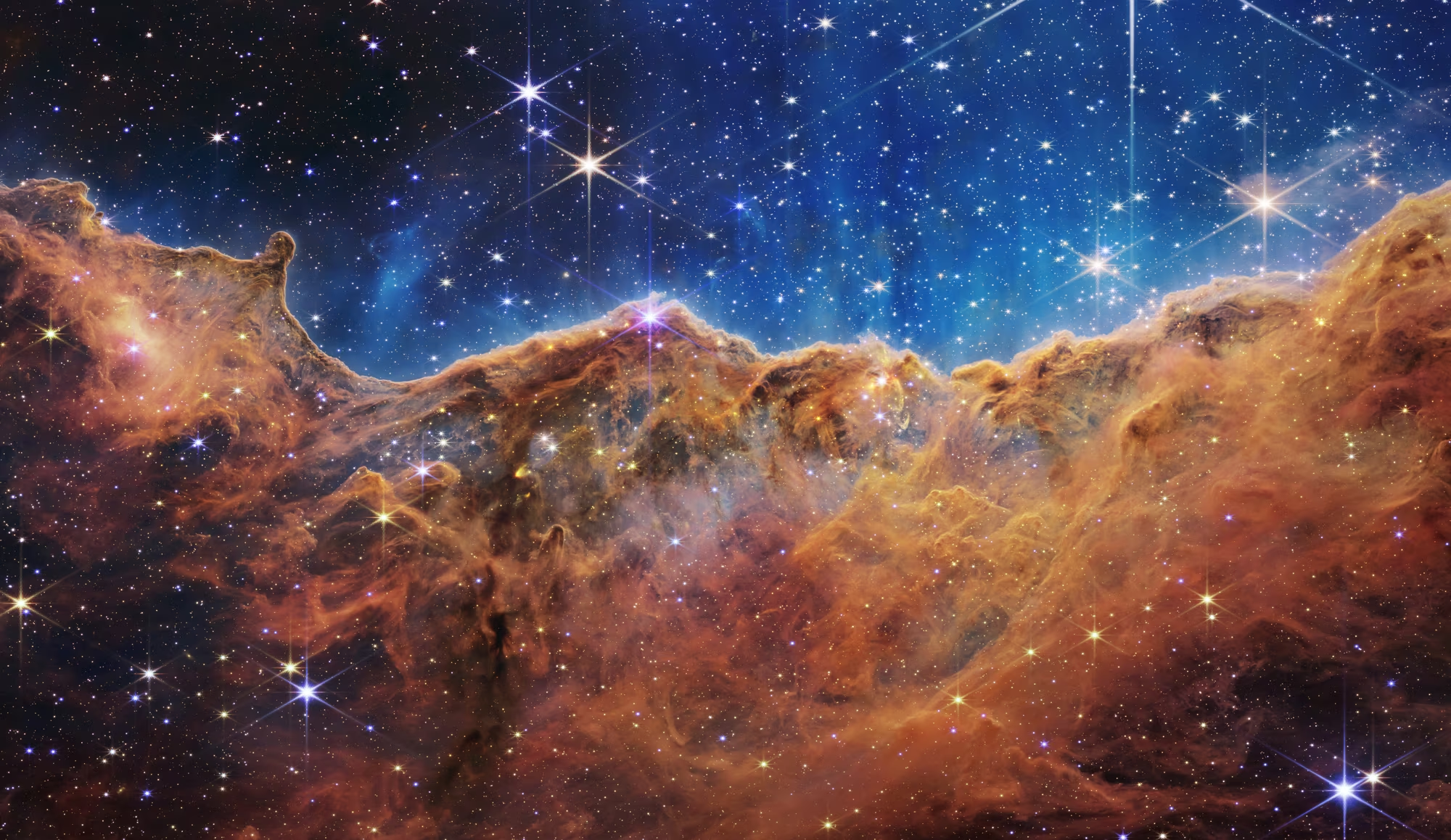
Fig. 2.1 The “Cosmic Cliffs” of the Carina Nebula imaged by JWST/NIRCam. Embedded protostars and outflows are visible at the edge of the molecular cloud where ultraviolet radiation from young massive stars sculpts the gas. Such regions are the present-day analogues of the environment in which the Solar System was born. Credit: NASA/ESA/CSA/STScI.

2.1.2. Disk structure and properties

Protoplanetary disks are not uniform: they have well-defined radial and vertical structure governed by the balance of gravity, pressure, and rotation:

• Temperature gradient: The disk is heated by stellar irradiation and viscous dissipation. Temperatures range from \(> 1500\) K in the innermost regions (where silicates are vaporised) to \(< 30\) K in the outer disk [Andrews, 2020]. This temperature profile determines which materials can condense as solids at each distance.

• Surface density: The mass distribution follows roughly a power-law profile \(\Sigma(r) \propto r^{-p}\) with \(p \approx 0.5\)–\(1.5\), meaning the surface density is highest in the inner disk (the integrated mass budget, by contrast, is dominated by the vastly larger area of the outer disk). Inferred disk masses decline from a few percent of the stellar mass in the youngest, embedded systems to of order \(0.1\)% by the Class II stage (the phase in which the envelope has cleared and the star is surrounded by a protoplanetary disk), although these estimates carry substantial systematic uncertainty [Miotello et al., 2023].

• Dust-to-gas ratio: In the interstellar medium, dust makes up about 1% of the total mass. In disks, this ratio can be locally enhanced by dust settling to the midplane and radial drift, with important consequences for planet formation.

• Vertical structure: The disk is geometrically thin, with a scale height \(H/r \sim 0.03\)–\(0.1\) that increases with distance (a “flared” disk). Dust settles toward the midplane due to the vertical component of the star’s gravity, creating a denser dust layer within the gas disk. The flared geometry and central dark midplane are directly visible in edge-on systems such as HH 30 (Fig. 2.2); a schematic summary of the radial-vertical structure is given in Fig. 2.3.

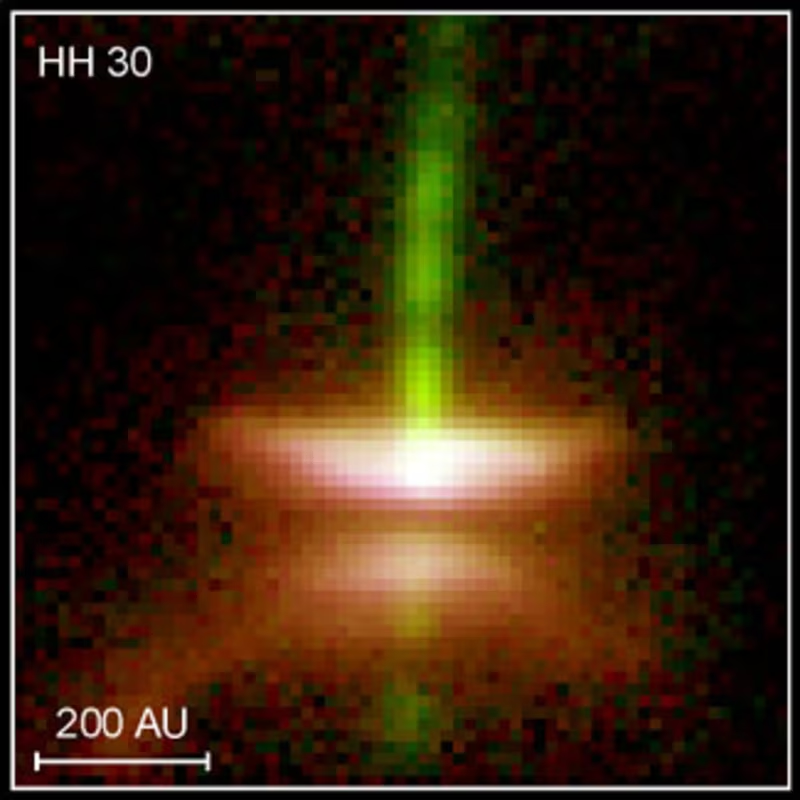
Fig. 2.2 Edge-on view of the embedded protoplanetary disk around HH 30, imaged by HST. The dark dust lane at the midplane and the bright bipolar nebulae illuminated by light scattering off the upper and lower disk surfaces directly visualise the flared, vertically thin geometry of a young protoplanetary disk. Credit: NASA/ESA/STScI.

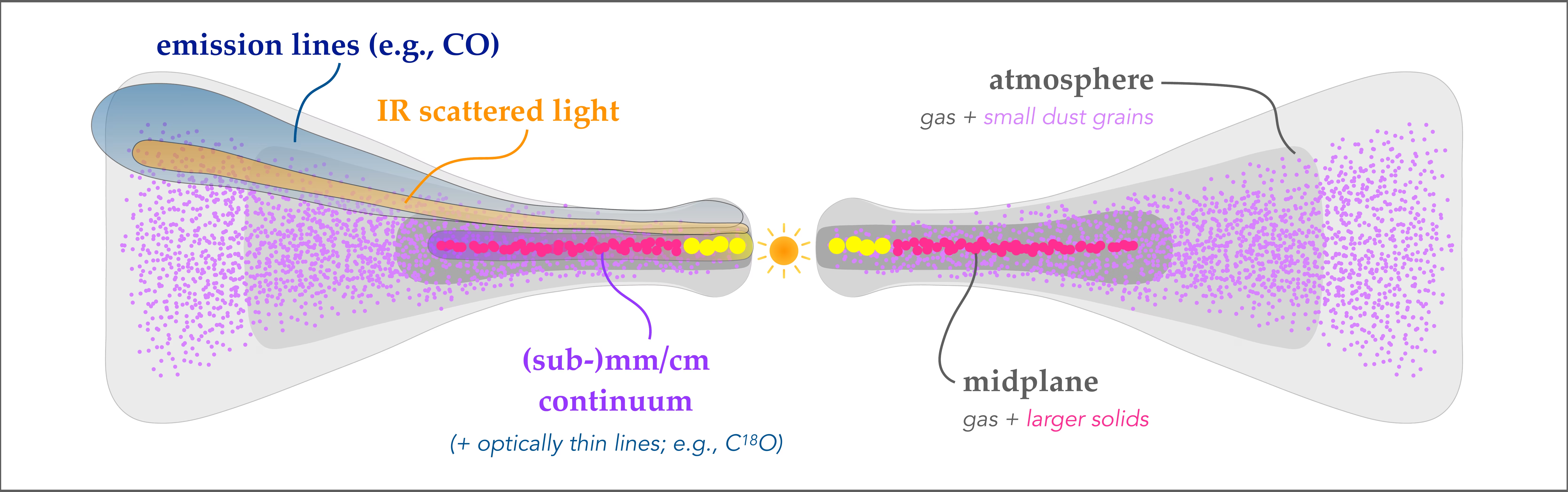
Fig. 2.3 Schematic cross-section of a protoplanetary disk. Gas is shown in grayscale and solids with exaggerated sizes; the flared geometry and the settling of larger solids to the dense midplane are directly visible. The left half labels the observational tracer of each region (\(\mathrm{CO}\) and other emission lines from the disk surface, infrared scattered light from small grains in the atmosphere, (sub-)mm/cm continuum from large grains near the midplane); the right half gives the structural vocabulary (gas atmosphere with small suspended grains, midplane layer of gas and larger solids). Adapted from Andrews [2020], Fig. 1; see also Williams and Cieza [2011] for an earlier review of disk structure.

2.1.3. The snow line and volatile distribution

A critical feature of any protoplanetary disk is the snow line (or ice line): the distance from the star beyond which water can condense as ice. In the solar nebula, this was located at roughly 2.5–3.5 AU, between the orbits of Mars and Jupiter. Quoted snow-line distances vary because the snow line moves: while the disk is young and accretion heating is strong it can sit out at \(\sim 5\) AU, and it migrates inward as the accretion rate declines and the disk cools [Drążkowska et al., 2023, Lichtenberg et al., 2021]; the 2.5–3.5 AU range is the location imprinted on the asteroid belt’s compositional gradient (Lecture 4, Lecture 12). The snow line matters because:

1. Beyond the snow line, solid material is much more abundant: adding water ice to the rocky/metallic inventory roughly triples the available solid mass.

2. The CHNOPS elements (carbon, hydrogen, nitrogen, oxygen, phosphorus, sulfur), essential for biology, are distributed between volatile and refractory phases depending on local disk temperature [Krijt et al., 2023]. The location where a planet forms relative to various ice lines determines its initial volatile budget.

Ice lines for other species (\(\mathrm{CO_2}\), \(\mathrm{CO}\), \(\mathrm{N_2}\), \(\mathrm{NH_3}\)) exist at progressively larger distances, creating a compositional gradient across the disk (Fig. 2.4).

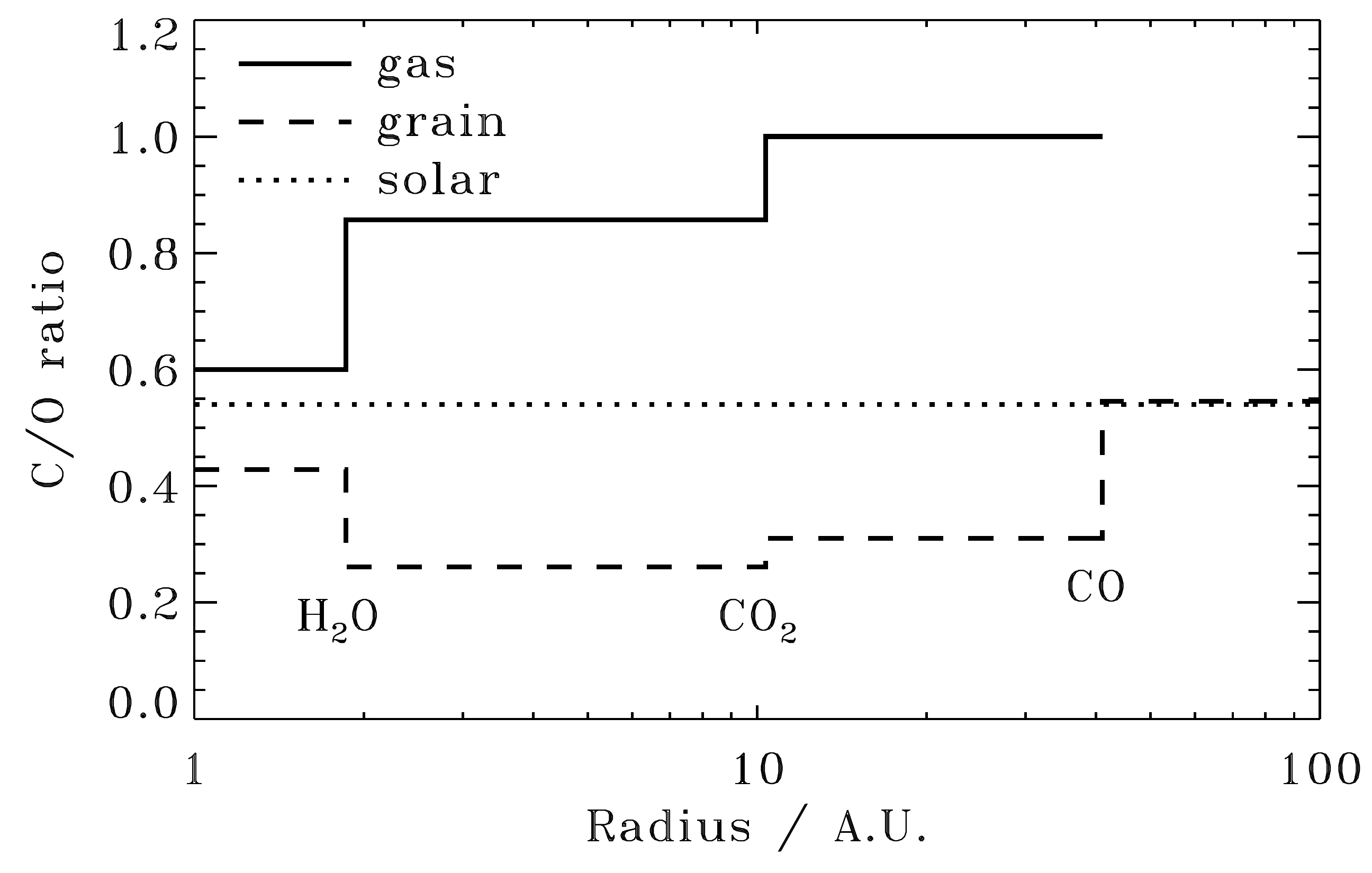
Fig. 2.4 Sequential condensation of major volatile species across a protoplanetary disk and the resulting C/O ratio of grains (dashed) and gas (solid) as a function of disk radius. The \(\mathrm{H_2O}\) ice line at \(\sim 2\) AU lowers grain C/O and raises gas C/O; beyond the \(\mathrm{CO_2}\) ice line at \(\sim 10\) AU the gas C/O reaches unity and holds that value out to the CO ice line at \(\sim 40\) AU, beyond which essentially all carbon and oxygen are frozen onto grains and the grain C/O returns to the stellar value (dotted line, solar C/O \(= 0.54\)). The radial sequencing of these ice lines controls the volatile composition that forming planets inherit from their formation zone. The exact \(\mathrm{H_2O}\) ice-line location is model-dependent and varies between \(\sim 2\) and \(3.5\) AU depending on the assumed disk temperature profile. Reproduced from Öberg et al. [2011], Fig. 1.

2.1.4. Observational evidence: ALMA

The Atacama Large Millimeter/submillimeter Array (ALMA) has revolutionised our understanding of protoplanetary disks. The landmark 2014 observation of HL Tauri (Fig. 2.5) revealed a young disk (\(\sim 1\) Myr) with a stunning series of concentric bright rings and dark gaps at AU-scale resolution [ALMA Partnership et al., 2015].

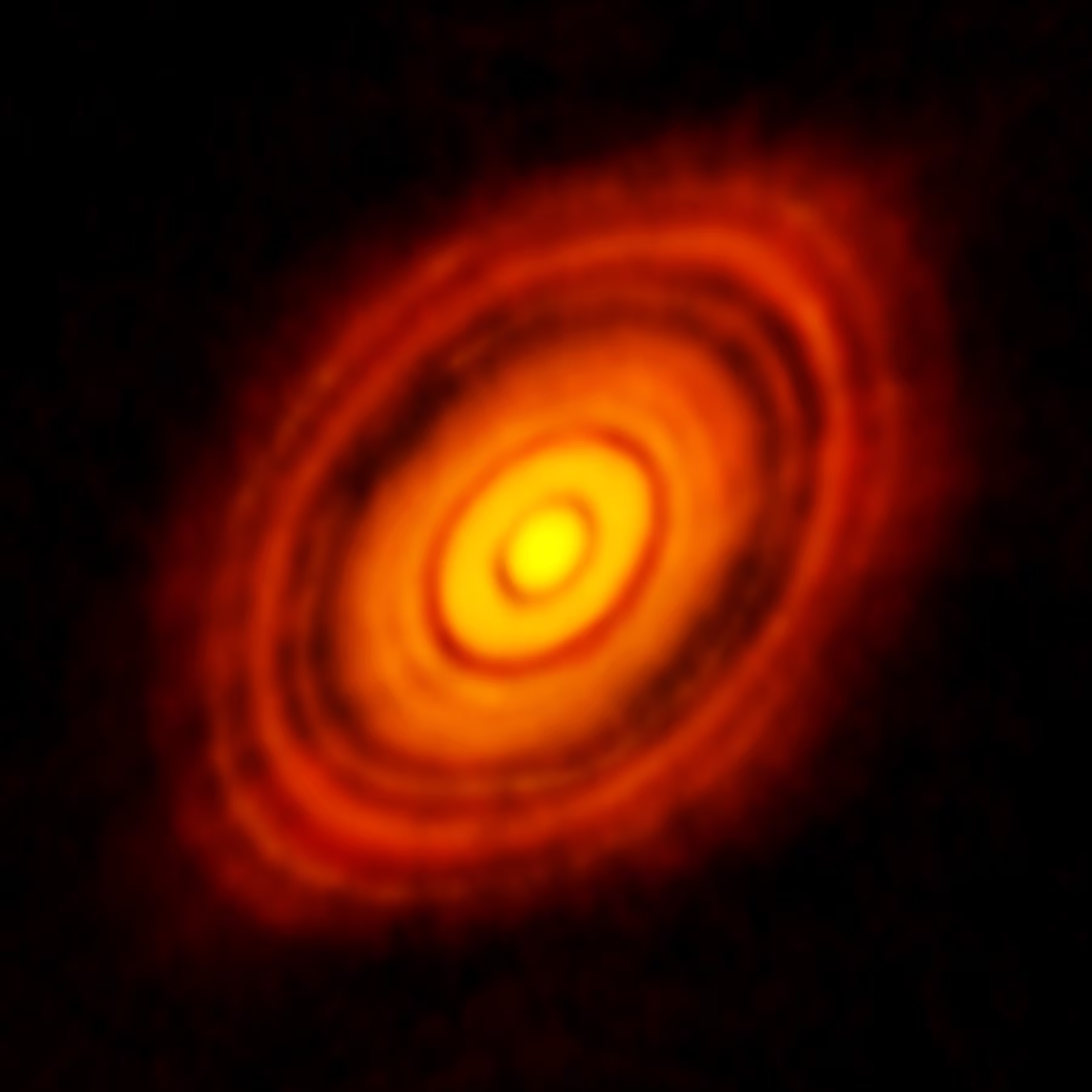
Fig. 2.5 ALMA image of the protoplanetary disk around HL Tauri, a young (\(\sim 1\) Myr) star in the Taurus molecular cloud, at 1.3 mm wavelength [ALMA Partnership et al., 2015]. The concentric bright rings and dark gaps extend to \(\sim 100\) AU. The gaps may be carved by forming planets, though other mechanisms (ice lines, magnetically driven structures) have also been proposed. Credit: ALMA (ESO/NAOJ/NRAO), CC BY 4.0.

The DSHARP survey (Disk Substructures at High Angular Resolution Project) extended this to 20 nearby disks (Fig. 2.6), revealing rings and gaps in every one of its targets [Andrews et al., 2018]. The sample was deliberately biased toward the largest and brightest disks, so not every disk need be so richly structured, but the result shows that the conditions for planet formation are established very early in disk evolution.

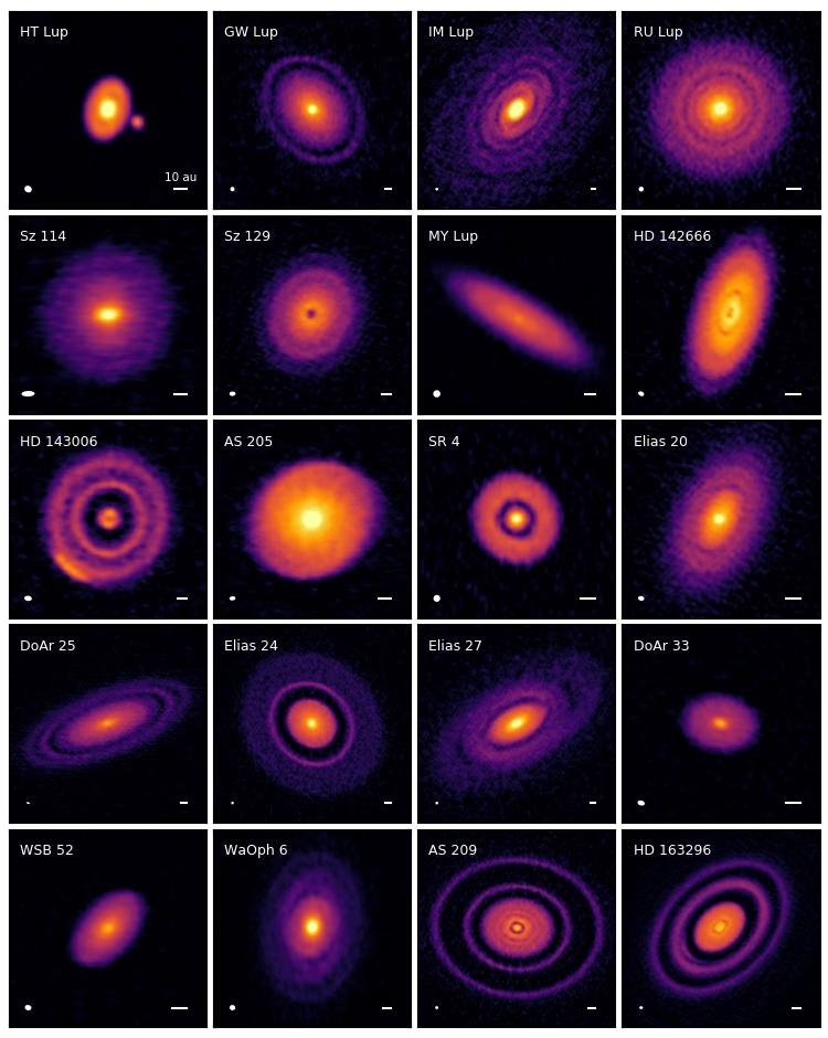
Fig. 2.6 Gallery of 240 GHz (\(1.25\) mm) continuum images of the 20 disks in the ALMA DSHARP sample, observed at \(\sim 5\) AU resolution. Beam sizes and \(10\) AU scale bars are shown in the lower left and right corners of each panel, and the colour stretch is chosen to bring out faint substructure. Rings and gaps appear in nearly every disk. Reproduced from Andrews et al. [2018], Fig. 3.

2.1.5. Disk lifetimes

Infrared excess surveys of young stellar clusters at different ages show that the fraction of stars retaining optically thick inner disks declines from \(\sim 80\)% at 1 Myr to \(< 10\)% by \(\sim 6\) Myr [Haisch et al., 2001]. Half of all stars lose their inner disks within \(\sim 3\) Myr, and essentially all disks are gone by \(\sim 6\) Myr (the \(\sim 1\)–\(3\) Myr protostellar accretion phase noted above is the earlier, embedded part of this lifetime). This sets a hard deadline for gas giant formation: if a planet’s core does not grow large enough to capture a gaseous envelope before the disk disperses, it will remain a rocky or icy body.

Disk dispersal is driven by a combination of viscous accretion onto the star, photoevaporation by stellar ultraviolet and X-ray radiation, and possibly magnetohydrodynamic winds.

2.2. Dust coagulation and planetesimal formation

The raw building material for planets consists of sub-micrometre dust grains (silicates, metal oxides, and, beyond the snow line, ices) embedded in the gas disk. Growing from micrometre-sized dust to thousand-kilometre planets is a factor of \(\sim 10^{12}\) in size, and the physics changes dramatically at each scale.

2.2.1. Grain growth: sticking and settling

In the dense midplane of the disk, dust grains collide due to Brownian motion, turbulence, and differential settling. At low velocities (\(\lesssim 1\) m s\(^{-1}\)), grains stick together through van der Waals forces, forming fractal aggregates: fluffy, porous structures that grow progressively larger (Fig. 2.7) [Blum and Wurm, 2008]. This process is efficient up to millimetre and centimetre sizes.

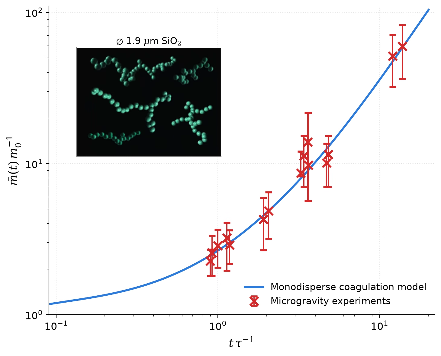
Fig. 2.7 Microgravity laboratory experiments on the earliest stage of dust coagulation. Inset: fractal aggregates (fractal dimension \(D \approx 1.4\)) of \(1.9\) µm \(\mathrm{SiO_2}\) monomers grown in space-shuttle experiments. Main panel: mean aggregate mass, in units of the monomer mass, versus time in units of the monomer collision timescale; the experimental points follow the solution of a monodisperse Smoluchowski coagulation model (curve) under Brownian-motion-driven sticking. Redrawn from Blum and Wurm [2008], Fig. 2; the data points and the model curve are digitized from the published figure.

2.2.2. Growth barriers

Beyond centimetre scales, several barriers impede further growth [Birnstiel et al., 2016]:

• Bouncing barrier (\(\sim\) mm): At slightly higher collision velocities, compacted aggregates bounce off each other rather than sticking, stalling growth at millimetre sizes.

• Fragmentation barrier (\(\sim\) cm): At collision velocities above \(\sim 1\)–\(10\) m s\(^{-1}\) (depending on material), aggregates shatter rather than merge. Silicate particles are particularly fragile; icy particles can survive higher-velocity impacts.

• Radial drift barrier (\(\sim\) metre): Solid particles orbiting in a gas disk experience a headwind because the gas, partially supported by its own pressure gradient, orbits slightly slower than the Keplerian velocity. This headwind causes particles to lose angular momentum and spiral inward. The drift rate peaks for metre-sized boulders, which would fall into the star in \(\sim 100\)–\(1000\) years, far faster than they can grow. This is the notorious metre-size barrier or radial drift barrier.

The combined effect of these barriers is summarised in Fig. 2.8: incremental sticking alone cannot bridge the gap between dust grains and planetesimals, motivating collective mechanisms such as the streaming instability discussed below.

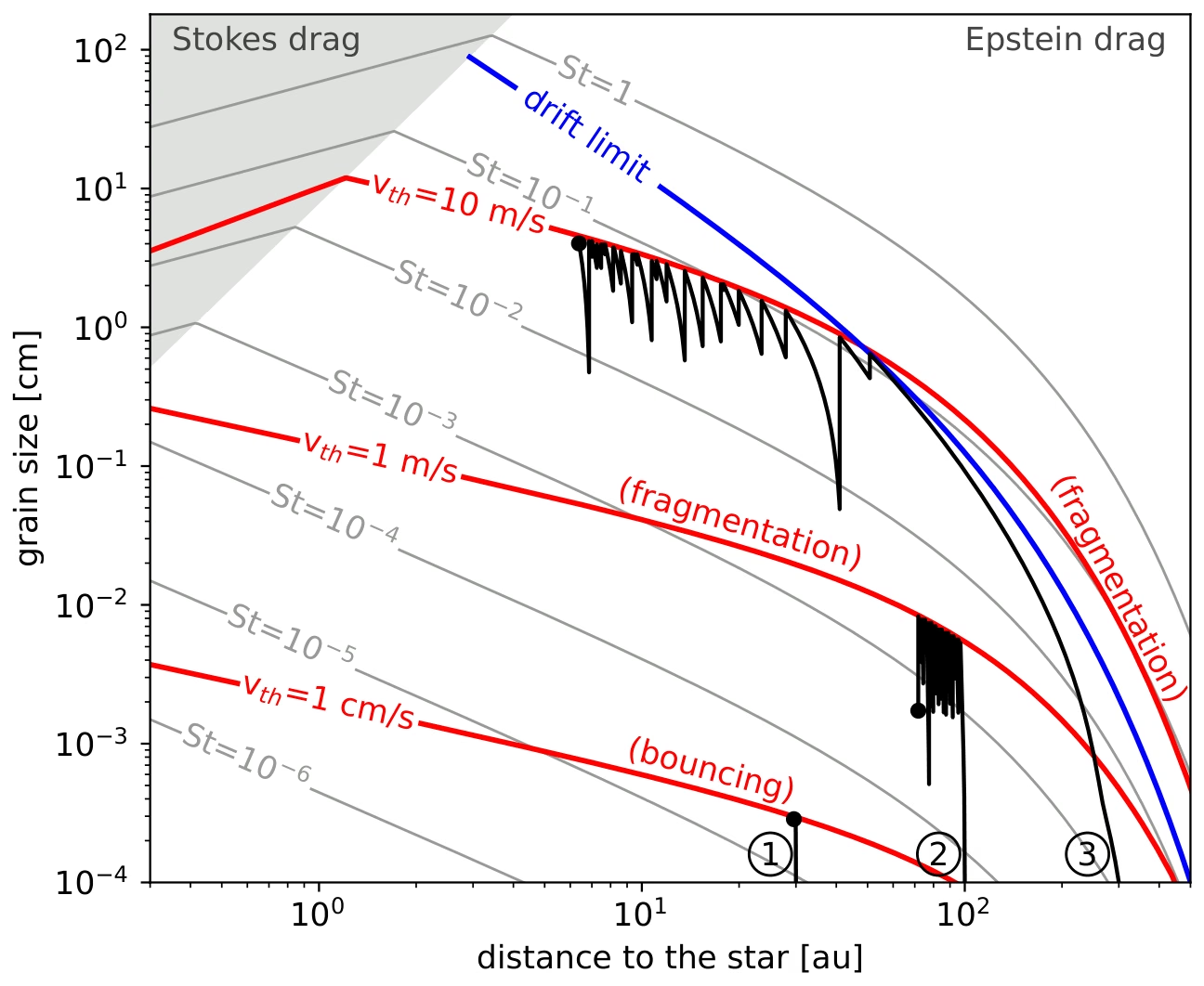
Fig. 2.8 Maximum grain size as a function of orbital distance in a standard disk model. Red curves mark the largest size that coagulation attains for three collision-velocity thresholds: bouncing at \(v_{\mathrm{th}} = 1\) cm s\(^{-1}\), and fragmentation at \(1\) and \(10\) m s\(^{-1}\). The blue curve is the radial-drift limit, above which grains drift inward faster than they grow; it does not apply inside the shaded Stokes-drag region at upper left, where growth is always faster than drift. Grey contours show constant Stokes number (the degree of aerodynamic coupling to the gas) from \(10^{-6}\) to unity. The three black curves are the growth tracks of test particles 1 to 3, whose sticking thresholds are \(1\) cm s\(^{-1}\), \(1\) m s\(^{-1}\) and \(10\) m s\(^{-1}\) respectively. Depending on location and material strength, incremental sticking stalls between tens of µm and dm sizes, far short of planetesimals, motivating collective mechanisms such as the streaming instability. Reproduced from Drążkowska et al. [2023], Fig. 4 (see also Birnstiel et al. [2016]).

2.2.3. The streaming instability

The solution to the radial drift problem appears to be collective effects. When the local dust-to-gas mass ratio approaches or exceeds unity (which can happen through settling to the midplane and accumulation at pressure bumps), the drag interaction between dust and gas changes qualitatively. Instead of all particles drifting inward, they can spontaneously clump through a process called the streaming instability [Johansen et al., 2007].

In the streaming instability, particles that happen to be concentrated accelerate the local gas toward the Keplerian velocity (reducing the headwind), which attracts more drifting particles from further out. This positive feedback loop creates dense filaments and clumps of pebbles (Fig. 2.9). When these clumps become sufficiently dense, they collapse under their own gravity to form planetesimals, solid bodies with radii from tens to a few hundred kilometres [Simon et al., 2016], essentially bypassing the difficult metre-to-kilometre growth step that direct sticking cannot achieve.

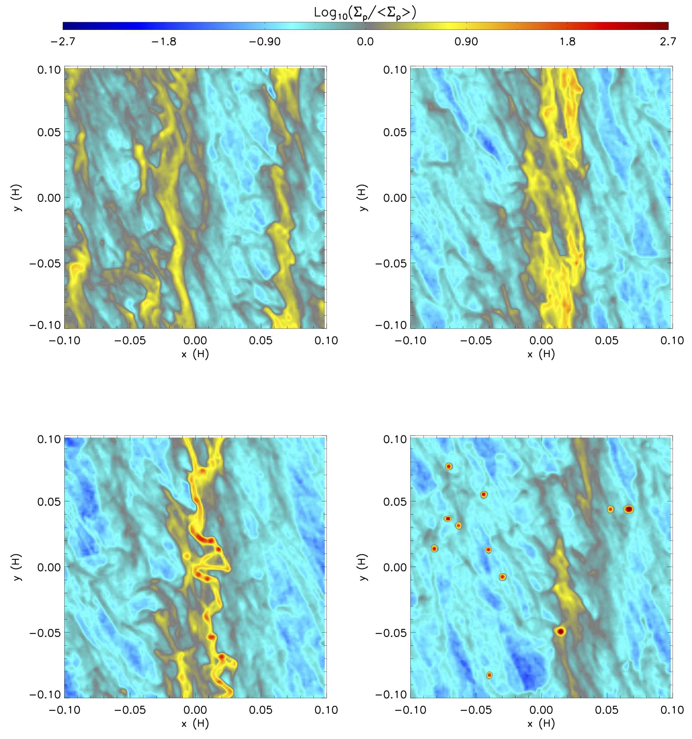
Fig. 2.9 Four snapshots of the particle surface density (normalised to its mean, logarithmic colour scale; axes in gas scale heights \(H\)) in a local shearing-box simulation of the streaming instability. Time increases from top left to bottom right: drag feedback concentrates the pebbles into dense, azimuthally extended filaments, which fragment under their own gravity; in the final snapshot the bound clumps (red points) have collapsed into planetesimals. Reproduced from Simon et al. [2016], Fig. 3.

2.2.4. Pebble accretion

Once planetesimals exist, those that are large enough can grow efficiently by sweeping up the abundant mm- to cm-sized “pebbles” that pervade the disk. This pebble accretion mechanism (Fig. 2.10) [Lambrechts and Johansen, 2012] is far more efficient than the classical picture of accreting only planetesimals, because gas drag causes pebbles to be strongly deflected toward the growing body, dramatically increasing the effective cross-section. Pebble accretion enables planetary cores to grow to \(\sim 10\) \(\Mearth\) within the disk lifetime, fast enough to trigger gas accretion and form giant planets. It is also self-limiting: once a planet grows massive enough, its gravity raises a pressure bump in the gas just outside its orbit that halts the inward pebble drift. Beyond this pebble isolation mass the planet’s pebble supply is cut off, and so is that of the entire disk interior to its orbit, a mechanism we will meet again in Lecture 12 [Drążkowska et al., 2023].

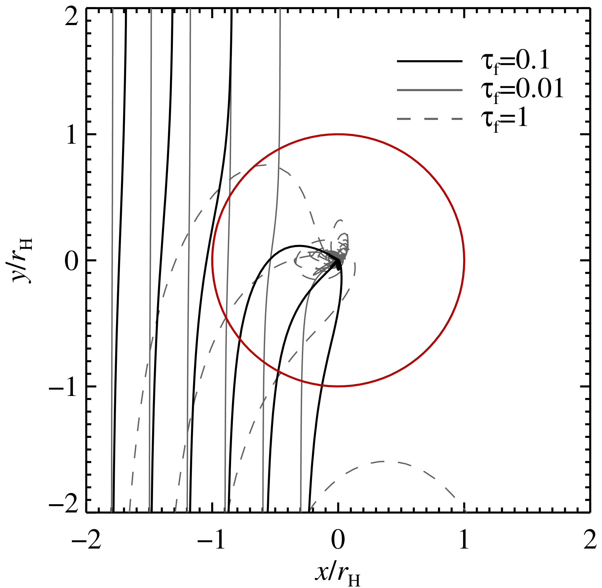
Fig. 2.10 Pebble trajectories around a growing planetary embryo, in the frame co-moving with the embryo (axes in units of the Hill radius \(r_{\mathrm{H}}\); the red circle marks the Hill sphere, inside which the embryo’s gravity dominates over the stellar tide). Line styles distinguish three dimensionless friction times (\(\tau_{\mathrm{f}} = 0.01\), \(0.1\), \(1\)), i.e. increasing degrees of decoupling from the gas. Gas drag causes pebbles entering the Hill sphere to lose angular momentum and spiral onto the embryo, enlarging the effective accretion cross-section far beyond the geometric value and allowing cores to reach \(\sim 10\,\Mearth\) within the disk lifetime. Reproduced from Lambrechts and Johansen [2012], Fig. 7.

2.2.5. Preferential formation sites

Planet formation does not proceed uniformly throughout the disk. Planets preferentially form at locations where conditions favour dust concentration: pressure bumps (where the gas pressure has a local maximum, halting radial drift), ice lines (where sublimation and recondensation enhance local solid density), and the edges of dead zones (regions of low turbulence). The resulting non-uniform distribution of forming planets helps explain the diverse architectures observed in exoplanetary systems [Drążkowska et al., 2023]. Fig. 2.11 summarises the modern roadmap from sub-µm dust to fully assembled planets.

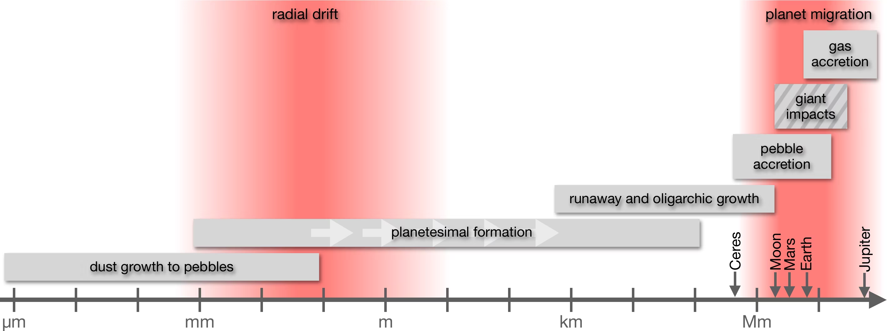
Fig. 2.11 Roadmap of the planet-formation sequence, organised by body size from sub-µm dust to gas giants (note the reference bodies Ceres, Moon, Mars, Earth, and Jupiter along the axis). Grey bars span the size range over which each process operates: dust growth to pebbles, planetesimal formation, runaway and oligarchic growth, pebble accretion, giant impacts, and gas accretion; the hatched giant-impact bar marks the one process that continues after the gas disk has dispersed. Red bands mark the two great obstacles: radial drift at pebble-to-boulder sizes and planet migration at planetary masses. Adapted from Drążkowska et al. [2023].

2.3. Runaway and oligarchic growth

Once a population of planetesimals has formed, gravitational interactions take over as the dominant growth mechanism.

2.3.1. Runaway growth

In a swarm of planetesimals, larger bodies have a decisive advantage: their stronger gravity allows them to focus incoming trajectories toward themselves, effectively increasing their collision cross-section far beyond their geometric size. The effective cross-section is enhanced by the gravitational focusing factor:

(2.2)\[ \sigma_{\mathrm{eff}} = \pi R^2 \left(1 + \frac{v_{\mathrm{esc}}^2}{v_{\infty}^2}\right) \]

where \(R\) is the body’s radius, \(v_{\mathrm{esc}} = \sqrt{2GM/R}\) is the escape velocity, and \(v_{\infty}\) is the relative velocity at infinity (approach velocity). When \(v_{\mathrm{esc}} \gg v_{\infty}\) (which occurs when the random velocities of planetesimals are small), the focusing factor can be enormous. Because \(v_{\mathrm{esc}}\) increases with mass, the largest body grows faster than its neighbours: this is runaway growth. A single body can rapidly outpace the rest of the swarm, reaching roughly lunar mass within \(\sim 10^5\) years at 1 AU [Kokubo and Ida, 1998]; growth toward Mars-mass embryos continues in the slower oligarchic phase described below, and assembling the final terrestrial planets takes far longer still (Lecture 4).

2.3.2. Oligarchic growth

Runaway growth is self-limiting. As the largest bodies grow, they gravitationally stir up the surrounding planetesimals, increasing the random velocities \(v_{\infty}\) and thereby reducing the gravitational focusing factor. Growth transitions to the oligarchic regime [Kokubo and Ida, 1998], in which a few dozen roughly equal-mass “oligarchs” dominate their local feeding zones, each separated by \(\sim 5\)–\(10\) mutual Hill radii. They continue to grow by accreting the remaining smaller planetesimals, but more slowly, until each reaches its isolation mass: the mass at which it has consumed all available material in its feeding zone. In the inner solar system, the isolation mass is \(\sim 0.01\)–\(0.1\) \(\Mearth\) [Kokubo and Ida, 1998], insufficient to explain the terrestrial planets.

2.3.3. Core accretion: building giant planets

The dominant model for giant planet formation is the core accretion model [Pollack et al., 1996]. In this scenario:

1. A solid core grows by accreting planetesimals and pebbles in the outer disk (beyond the snow line, where more solid material is available).

2. Once the core reaches a critical mass of \(\sim 10\)–\(20\) \(\Mearth\), its gravity becomes strong enough to bind a substantial gas envelope from the surrounding disk.

3. The envelope contracts and cools, allowing more gas to flow in, leading to a phase of rapid, runaway gas accretion. Within \(\sim 10^5\) years, the planet can accumulate hundreds of Earth masses of hydrogen and helium.

4. Accretion ceases when the planet opens a gap in the disk or when the disk itself dissipates.

This model naturally explains why Jupiter and Saturn are massive (they formed in the solid-rich region beyond the snow line and reached critical core mass before disk dispersal) and why Uranus and Neptune are smaller (they likely reached critical mass too late, after most gas had been removed). The mass-vs-time evolution of the three core-accretion phases is shown in Fig. 2.12.

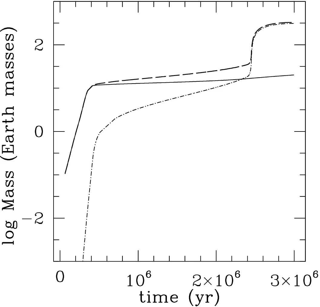
Fig. 2.12 Growth of a giant planet by core accretion, from a classic simulation of Jupiter’s formation at \(5.2\) AU in the framework of Pollack et al. [1996]. Solid line: core mass; dash-dotted line: envelope mass; dashed line: total mass. The three phases are clearly visible: rapid core growth to \(\sim 10\,\Mearth\) (Phase 1), a long plateau of slow, quasi-hydrostatic envelope growth (Phase 2), and runaway gas accretion after the envelope mass overtakes the core mass at the crossover point, at \(2.3\) Myr in this run, reaching a Jupiter mass by \(3\) Myr (Phase 3). Reproduced from Helled et al. [2014], Fig. 1; simulation from Lissauer et al. [2009].

2.3.4. Gravitational instability: an alternative pathway

An alternative scenario for gas giant formation is direct gravitational instability of the gas disk [Boss, 1997]. If a massive disk cools sufficiently rapidly, it can fragment into self-gravitating clumps that contract directly into giant planets, bypassing the slow step of building a solid core. This mechanism can form giant planets very quickly (on orbital timescales, \(\sim 10^3\) years), but the required conditions of high disk mass and efficient cooling are only realised at large orbital distances (\(\gtrsim 30\)–\(50\) AU) in unusually massive disks [Kratter and Lodato, 2016], so it is today considered a pathway for massive companions on wide orbits rather than for the solar system’s giant planets.

2.3.5. The giant impact phase

In the inner solar system, after the disk has dispersed and gas drag is no longer available to circularise orbits, the protoplanetary embryos (oligarchs) undergo a final phase of chaotic giant impacts lasting \(\sim 10\)–\(100\) Myr. Their orbits become increasingly eccentric and crossing, leading to collisions that assemble the final terrestrial planets from a smaller number of embryos. The Moon-forming impact (a collision between the proto-Earth and a Mars-sized body, Theia) is the most dramatic example from our solar system.

2.3.6. Geophysical evolution during formation

Planet formation is not merely an assembly process: it drives profound geophysical changes. The energy delivered by accretion and giant impacts melts the growing planet, producing a global magma ocean. In this molten state, dense metallic iron sinks to form a core, while lighter silicates float to form the mantle, a process called core-mantle differentiation. Early radioactive heating from short-lived isotopes (particularly \({}^{26}\mathrm{Al}\), with a half-life of 0.72 Myr) can melt even small planetesimals, initiating differentiation before the planet has finished assembling [Lichtenberg et al., 2023]. The thermal and chemical state inherited from this formation epoch profoundly shapes a planet’s subsequent evolution: its magnetic field, volcanic activity, atmospheric outgassing, and ultimately its habitability (Lecture 3, Lecture 4).

2.4. Kepler’s laws and orbital elements

Having discussed how planets form, we now turn to how they move. Planetary orbits are the most precisely measured quantities in all of planetary science, and they are governed by some of the simplest equations in physics.

2.4.1. Kepler’s three laws

In the early 17th century, Johannes Kepler distilled decades of precise observations by Tycho Brahe into three empirical laws:

1. The law of ellipses: Each planet moves in an elliptical orbit with the Sun at one focus.

2. The law of equal areas: A line connecting the planet to the Sun sweeps out equal areas in equal times. This means the planet moves fastest at perihelion (closest approach) and slowest at aphelion (farthest distance). For an orbit around an arbitrary central body these two turning points are called the periapsis and the apoapsis, together the apsides.

3. The harmonic law: The square of the orbital period is proportional to the cube of the semi-major axis:

(2.3)\[ P^2 = \frac{4\pi^2}{G(M_1 + M_2)}\, a^3 \]

As we saw in Lecture 1, Newton showed that all three laws follow from his universal law of gravitation. Kepler’s third law, in its Newtonian form (Eq. (2.3)), is one of the most useful equations in astronomy: it connects an easily measured quantity (the orbital period) to the total mass of the system. The geometry of the three laws is summarised in Fig. 2.13, and the resulting solar-system architecture, with all eight planets plus the asteroid belt and Kuiper Belt on a logarithmic semi-major-axis scale, is shown in Fig. 2.14.

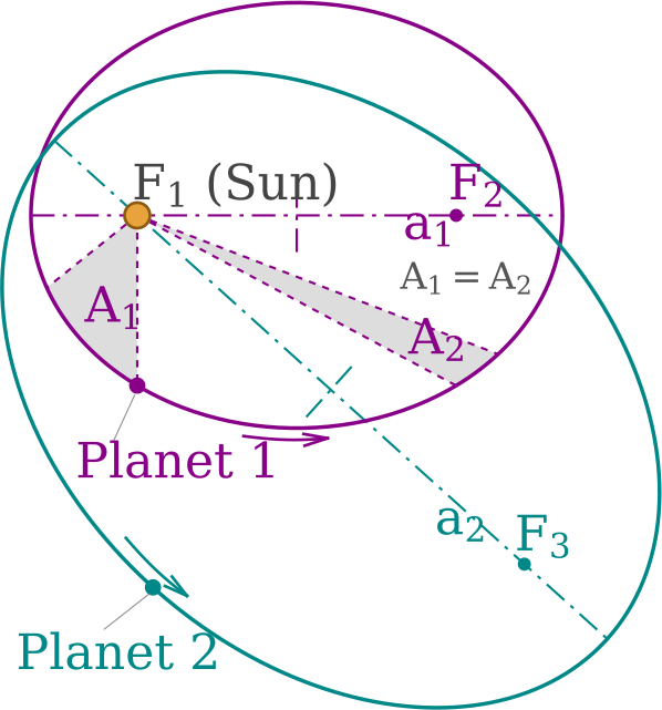
Fig. 2.13 Illustration of Kepler’s three laws of planetary motion. (1) Orbits are ellipses with the Sun at one focus; (2) the radius vector sweeps out equal areas in equal times (shaded regions have equal area); (3) the period-squared is proportional to the semi-major axis cubed. Redrawn after Hankwang (Wikimedia Commons), CC BY 2.5.

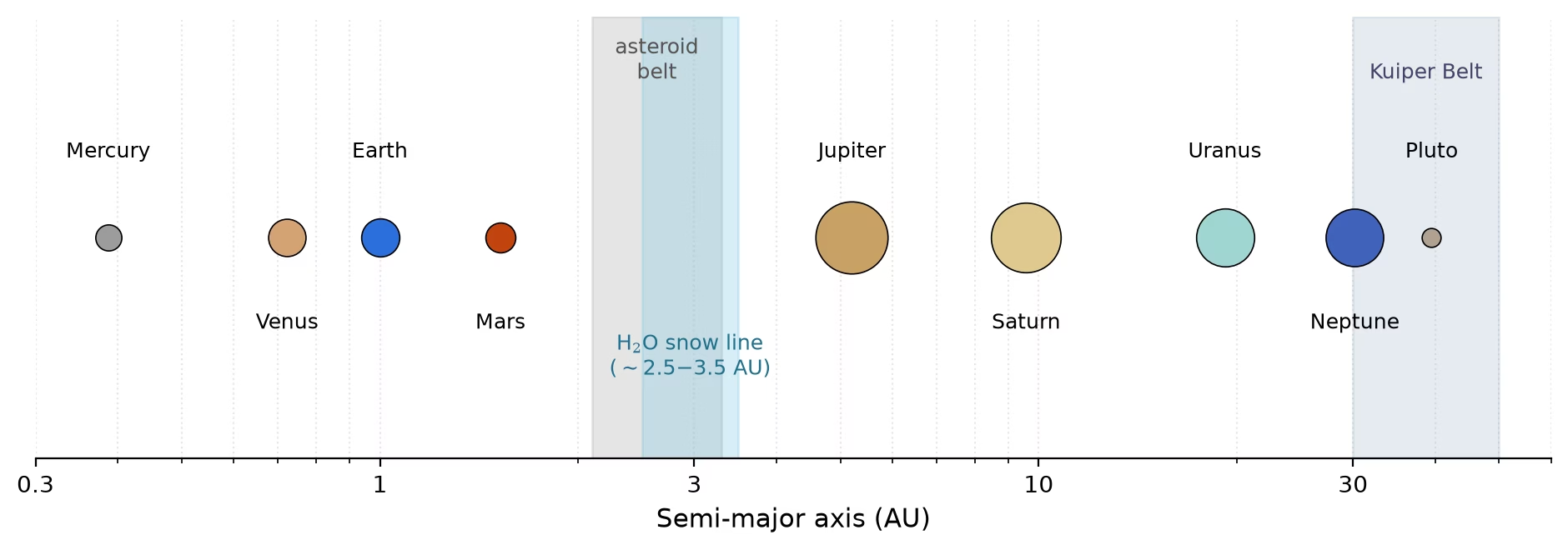
Fig. 2.14 Architecture of the Solar System on a logarithmic semi-major-axis scale. The eight planets and Pluto are drawn with symbol area scaled as \(\log(1 + R/R_\oplus)\) so that all bodies remain visible; shaded spans mark the asteroid main belt (\(2.1\)–\(3.3\) AU), the classical Kuiper Belt (\(30\)–\(50\) AU), and the \(2.5\)–\(3.5\) AU range in which the solar nebula’s water snow line lay, separating the rocky inner planets from the gas and ice giants. Semi-major axes and radii from Williams [2026]. Course-original figure.

2.4.2. Orbital elements

The orbit of a body in a gravitational field is fully described by six orbital elements:

Element	Symbol	Description
Semi-major axis	\(a\)	Size of the orbit (half the long axis of the ellipse)
Eccentricity	\(e\)	Shape of the orbit (\(e = 0\) is circular, \(0 < e < 1\) is elliptical)
Inclination	\(i\)	Tilt of the orbital plane relative to a reference plane
Longitude of ascending node	\(\Omega\)	Orientation of the line where the orbital plane crosses the reference plane
Argument of perihelion	\(\omega\)	Orientation of the ellipse within the orbital plane
True anomaly	\(\nu\)	Position of the body along the orbit at a given time

The first five elements define the size, shape, and orientation of the orbit; the sixth specifies where the body is at any moment. The geometric meaning of the four angular elements is illustrated in Fig. 2.15; the remaining two, \(a\) and \(e\), set the size and shape of the ellipse itself.

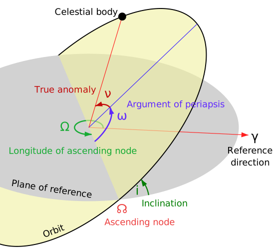
Fig. 2.15 The four angular orbital elements. The reference plane is shown in grey; the orbital plane is tilted by the inclination \(i\). The ascending node (\(\Omega\)) and argument of perihelion (\(\omega\); labelled “argument of periapsis” in the figure, the general term) orient the orbit in space, and the true anomaly (\(\nu\)) locates the body along it. Credit: Lasunncty, CC BY-SA 3.0.

In the solar system, most planets have nearly circular orbits (\(e < 0.1\)) and low inclinations (\(i \lesssim 3.5^{\circ}\)), which reflects the disk-like origin of the system. Exceptions include Mercury (\(e = 0.206\), \(i = 7.0^{\circ}\)) and, among dwarf planets, Pluto (\(e = 0.25\), \(i = 17^{\circ}\)), hinting at a more complex dynamical history.

2.5. Two-body problem and the vis-viva equation

2.5.1. The two-body problem

Consider two bodies of masses \(m_1\) and \(m_2\) interacting through gravity alone. In the centre-of-mass frame, the problem reduces to a single body of reduced mass

\[ \mu = \frac{m_1 m_2}{m_1 + m_2} \]

moving in the gravitational field of a fixed central mass \(M = m_1 + m_2\).

The total orbital energy is the sum of kinetic and gravitational potential energy:

\[ E = \frac{1}{2}\mu v^2 - \frac{G m_1 m_2}{r} \]

A fundamental result of orbital mechanics is that the total energy depends only on the semi-major axis:

(2.4)\[ E = -\frac{G m_1 m_2}{2a} \]

This means that two orbits with the same semi-major axis have the same total energy, regardless of their eccentricity. A circular orbit and a highly eccentric orbit with the same \(a\) are energetically equivalent: they simply distribute kinetic and potential energy differently along the orbit.

2.5.2. The vis-viva equation

Combining the total energy expression (Eq. (2.4)) with the instantaneous kinetic and potential energy, we obtain the vis-viva equation (Latin for “living force”):

(2.5)\[ \boxed{v^2 = G(m_1 + m_2)\left(\frac{2}{r} - \frac{1}{a}\right)} \]

For the common case where \(m_2 \ll m_1\) (e.g., a planet orbiting a star), this simplifies to:

\[ v^2 = GM\left(\frac{2}{r} - \frac{1}{a}\right) \]

Equation (2.5) tells us the speed \(v\) of an orbiting body at any distance \(r\) from the central mass, given the semi-major axis \(a\). It has important special cases:

• Circular orbit (\(r = a\)): \(v_{\mathrm{circ}} = \sqrt{GM/a}\)

• Escape velocity (\(a \to \infty\), \(E = 0\)): \(v_{\mathrm{esc}} = \sqrt{2GM/r}\)

The escape velocity is exactly \(\sqrt{2}\) times the circular orbital velocity at the same distance, a factor worth remembering.

2.6. Blackboard derivation: The vis-viva equation

Blackboard derivation: The vis-viva equation

Goal: Derive the vis-viva equation from energy conservation in a Keplerian orbit, then apply it to calculate orbital velocities for Earth and Halley’s comet.

Setup.

Consider a planet of mass \(m\) in an elliptical orbit around a star of mass \(M\) (with \(m \ll M\)). The orbit has semi-major axis \(a\) and eccentricity \(e\). At any point, the planet is at distance \(r\) from the star and moves with speed \(v\).

The total mechanical energy is conserved:

\[ E = \frac{1}{2}mv^2 - \frac{GMm}{r} = \mathrm{constant} \]

We want to express \(E\) in terms of \(a\) alone, then derive a formula for \(v(r)\).

Derivation.

Step 1: Evaluate energy at perihelion and aphelion.

At perihelion (closest approach), \(r_p = a(1 - e)\), and at aphelion (farthest distance), \(r_a = a(1 + e)\). Writing energy conservation at these two points:

\[ \frac{1}{2}mv_p^2 - \frac{GMm}{a(1-e)} = \frac{1}{2}mv_a^2 - \frac{GMm}{a(1+e)} \]

Step 2: Use angular momentum conservation.

At perihelion and aphelion, the velocity is purely tangential (perpendicular to the radius vector), so angular momentum conservation gives:

\[ L = m\, v_p\, r_p = m\, v_a\, r_a \quad \Rightarrow \quad v_p\, a(1-e) = v_a\, a(1+e) \]

Therefore \(v_p / v_a = (1+e)/(1-e)\).

Step 3: Solve for the total energy.

Substitute \(v_p = v_a\,(1+e)/(1-e)\) from Step 2 into the energy equality of Step 1, after dividing every term by \(m\):

\[ \frac{1}{2}v_a^2\,\frac{(1+e)^2}{(1-e)^2} - \frac{GM}{a(1-e)} = \frac{1}{2}v_a^2 - \frac{GM}{a(1+e)} \]

Collect the kinetic terms on the left and the potential terms on the right:

\[ \frac{1}{2}v_a^2\left[\frac{(1+e)^2 - (1-e)^2}{(1-e)^2}\right] = \frac{GM}{a}\left[\frac{1}{1-e} - \frac{1}{1+e}\right] \]

Both brackets collapse: \((1+e)^2 - (1-e)^2 = 4e\), and \(1/(1-e) - 1/(1+e) = 2e/[(1-e)(1+e)]\), so

\[ \frac{2e\,v_a^2}{(1-e)^2} = \frac{GM}{a}\,\frac{2e}{(1-e)(1+e)} \]

Divide both sides by \(2e/(1-e)^2\) (taking \(e \neq 0\); for \(e = 0\) the two apsides coincide, the orbit is circular, and the result of Step 4 follows directly from the force balance of Lecture 1):

\[ v_a^2 = \frac{GM}{a}\,\frac{1-e}{1+e} \]

Insert this into the total energy evaluated at aphelion:

\[\begin{split} \begin{aligned} \frac{E}{m} &= \frac{1}{2}v_a^2 - \frac{GM}{a(1+e)} = \frac{GM}{2a}\,\frac{1-e}{1+e} - \frac{GM}{a(1+e)} \\ &= \frac{GM}{a(1+e)}\left[\frac{1-e}{2} - 1\right] = -\frac{GM}{a(1+e)}\,\frac{1+e}{2} \end{aligned} \end{split}\]

\[ E = -\frac{GMm}{2a} \]

This is a remarkable result: the total energy depends only on the semi-major axis, not on the eccentricity.

Step 4: Write the vis-viva equation.

Setting the total energy equal to the instantaneous kinetic + potential energy:

\[ \frac{1}{2}mv^2 - \frac{GMm}{r} = -\frac{GMm}{2a} \]

Dividing through by \(m/2\) and rearranging:

\[ \boxed{v^2 = GM\left(\frac{2}{r} - \frac{1}{a}\right)} \]

Application: Earth’s orbital velocity.

For Earth (\(a = 1\) AU \(= 1.496 \times 10^{11}\) m, \(e = 0.0167\)):

Point	Distance \(r\)	Velocity
Perihelion	\(a(1-e) = 1.471 \times 10^{11}\) m	\(v_p = 30.29\) km s\(^{-1}\)
Aphelion	\(a(1+e) = 1.521 \times 10^{11}\) m	\(v_a = 29.29\) km s\(^{-1}\)

The variation is only about \(\pm 0.5\) km s\(^{-1}\) around the mean, because Earth’s orbit is nearly circular. The mean orbital velocity is approximately \(v \approx 2\pi a / P \approx 29.8\) km s\(^{-1}\).

Application: Halley’s comet.

For a dramatic contrast, consider Halley’s comet (\(a = 17.83\) AU, \(e = 0.967\)):

Point	Distance \(r\)	Velocity
Perihelion	\(a(1-e) = 0.588\) AU	\(v_p = 54.5\) km s\(^{-1}\)
Aphelion	\(a(1+e) = 35.1\) AU	\(v_a = 0.91\) km s\(^{-1}\)

Halley’s comet hurtles through the inner solar system at nearly twice Earth’s speed, yet crawls beyond Neptune’s orbit at less than 1 km s\(^{-1}\). This enormous range is a direct consequence of the vis-viva equation applied to a highly eccentric orbit; both speed profiles are plotted in Fig. 2.16.

Note: The vis-viva equation generalises the circular-orbit force balance of Lecture 1: there, setting the gravitational attraction equal to the centripetal acceleration gave \(v^2 = GM/r\), which is the vis-viva equation for the special case \(r = a\).

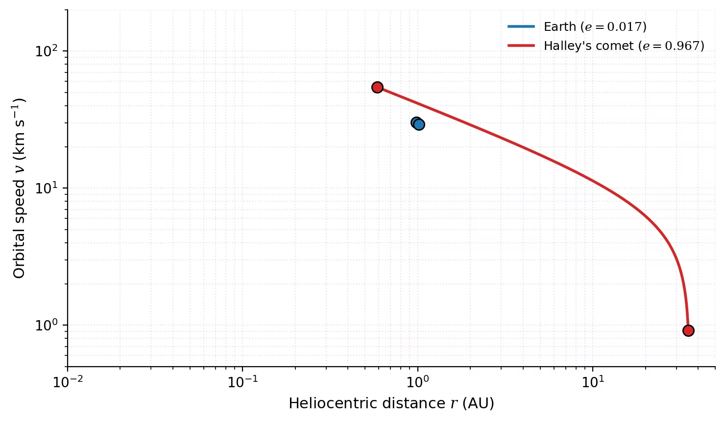
Fig. 2.16 Orbital speed \(v(r)\) from the vis-viva equation for Earth (\(a = 1\) AU, \(e = 0.0167\)) and Halley’s comet (\(a = 17.83\) AU, \(e = 0.967\)). Filled circles mark perihelion and aphelion of each orbit. Earth’s nearly circular orbit gives \(v \approx 30\) km s\(^{-1}\) throughout, whereas Halley’s high eccentricity produces a \(\sim 60\times\) swing in speed between perihelion (\(54.5\) km s\(^{-1}\)) and aphelion (\(0.91\) km s\(^{-1}\)). Course-original figure.

2.7. Orbital resonances

When two orbiting bodies have orbital periods in a ratio of small integers, they are in a mean-motion resonance (MMR). At each conjunction (closest approach), the bodies are at the same relative positions, and their mutual gravitational perturbations add up coherently over many orbits, rather than averaging to zero.

2.7.1. Mean-motion resonances

A \(p\):\(q\) mean-motion resonance (with \(p > q\)) means that the inner body completes \(p\) orbits in the same time the outer body completes \(q\) orbits. The gravitational kicks at each conjunction always occur at the same orbital phases, which can either stabilise or destabilise the configuration depending on the geometry [Murray and Dermott, 1999].

Resonances are widespread in the solar system:

Resonance	Bodies	Period ratio
3:2	Pluto-Neptune	Pluto completes 2 orbits per 3 of Neptune
Near 5:2	Jupiter-Saturn	“Great inequality”: near-resonance drives long-period perturbations
3:1, 5:2, 7:3, 2:1	Several asteroid gaps	Kirkwood gaps in the asteroid belt (Lecture 12)
1:1	Jupiter Trojans	Co-orbital asteroids at L4 and L5 Lagrange points

2.7.2. The Laplace resonance

The most famous resonance in the solar system is the Laplace resonance of Jupiter’s three inner Galilean moons: Io, Europa, and Ganymede. Their orbital periods are in a 1:2:4 ratio (equivalently, mean motions \(n \equiv 2\pi/P\), the orbital angular frequencies, in the ratio \(n_{\mathrm{Io}} : n_{\mathrm{Eur}} : n_{\mathrm{Gan}} = 4:2:1\); Io completes four orbits for each orbit of Ganymede):

Moon	Period (days)	Ratio to Io
Io	1.769	1
Europa	3.551	\(\approx\) 2
Ganymede	7.155	\(\approx\) 4

This three-body resonance is maintained by tidal interactions with Jupiter. The key consequence is that it forces non-zero orbital eccentricities: Io’s eccentricity is maintained at \(e \approx 0.004\) (small, but crucial) [Peale et al., 1979]. This continual eccentricity forcing drives tidal flexing inside Io, generating enough heat to make it the most volcanically active body in the solar system (Fig. 2.17, Fig. 2.18), a connection we will explore in Lecture 3.

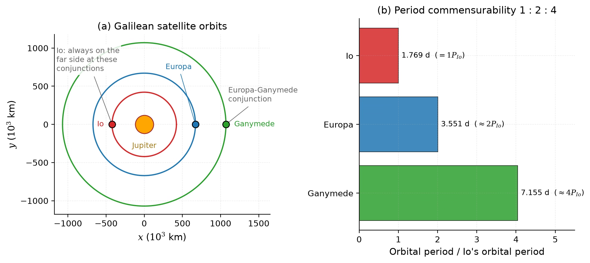
Fig. 2.17 The Laplace resonance of the Galilean moons. Panel (a): the orbits of Io, Europa, and Ganymede to scale, drawn at a Europa-Ganymede conjunction; the resonance locks the moons’ phases such that Io is always on the opposite side of Jupiter at these conjunctions, so a triple conjunction never occurs. Panel (b): the orbital periods stand in the ratio 1 : 2 : 4, and the pattern of successive conjunctions repeats every Ganymede period (four Io orbits). The resulting periodic gravitational kicks force a non-zero eccentricity on Io (\(e \approx 0.004\)), driving the tidal heating that powers its volcanism [Peale et al., 1979]. Course-original figure.

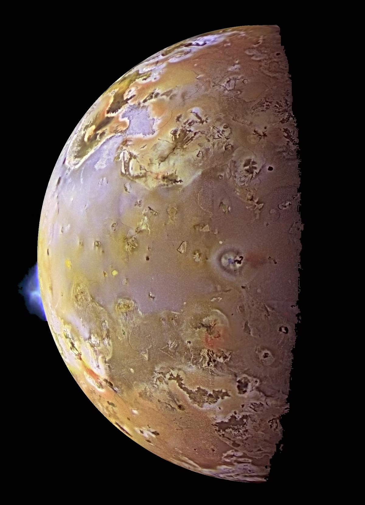
Fig. 2.18 Half-disk view of Jupiter’s moon Io imaged by the Galileo spacecraft, showing an active volcanic plume rising in profile against the dark sky at the limb. The mottled, sulfur-rich surface is reshaped on geological timescales by the underlying volcanism. Resonance-forced eccentricity from the Laplace resonance feeds tidal dissipation that makes Io the most volcanically active body in the Solar System. Credit: NASA/JPL/University of Arizona.

2.8. Tidal forces and tidal locking

2.8.1. The tidal force

A tidal force arises whenever a gravitational field varies across the finite extent of an extended body. Consider a moon of radius \(R_s\) at distance \(d\) from a planet of mass \(M_p\). The near side of the moon experiences a stronger gravitational pull than the far side, creating a differential force that tends to elongate the moon along the line connecting it to the planet. The tidal acceleration between the moon’s centre and its near side is approximately:

\[ \Delta a_{\mathrm{tidal}} \approx \frac{2 G M_p R_s}{d^3} \]

This \(1/d^3\) dependence (compared to the \(1/d^2\) dependence of gravity itself) means that tidal forces are strongly distance-dependent.

2.8.2. Tidal bulges and energy dissipation

The tidal force raises tidal bulges on both sides of the body: one facing the perturber and one on the opposite side. If the body rotates at a different rate than it orbits (which is initially the case for most moons and planets), the bulges are carried away from the line connecting the two bodies. This misalignment creates a torque that transfers angular momentum between the body’s spin and its orbit, gradually changing both. The energy dissipated in continually deforming the body is converted to heat: this is tidal heating, which powers Io’s volcanism and may maintain subsurface oceans on Europa and Enceladus (Lecture 3).

2.8.3. Tidal locking (synchronous rotation)

Over time, the tidal torque slows the faster-spinning body until its rotation period equals its orbital period, a state called synchronous rotation or tidal locking (Fig. 2.19). In this configuration, the same face always points toward the perturber, and the tidal bulge is aligned with the connecting line, so no further torque acts. Synchronous rotation does not switch off tidal dissipation entirely, however: on an eccentric orbit the distance to the perturber and the apparent direction of the bulge vary over each orbit, so a locked body continues to flex and heat. This is precisely Io’s situation: its eccentricity, pinned at \(e \approx 0.004\) by the Laplace resonance, sustains the tidal heating behind its volcanism (Lecture 3).

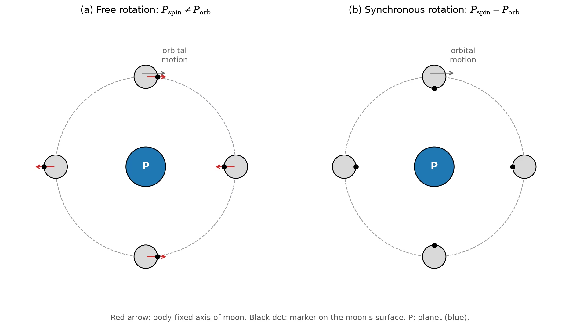
Fig. 2.19 Free versus synchronous rotation. Panel (a): a moon whose spin period differs from its orbital period shows different faces to the planet (P) over one orbit; the black surface marker and the body-fixed axis (red arrow) decouple from the direction to the planet. Panel (b): in synchronous rotation the spin and orbital periods are equal, so the surface marker, and with it the tidal bulge, always faces the planet. The Moon reached this state through billions of years of tidal dissipation [Murray and Dermott, 1999]. Course-original figure.

The Moon is tidally locked to Earth; this is why we always see the same face. All four Galilean moons are tidally locked to Jupiter. Most large moons in the solar system are synchronous rotators. The timescale for tidal locking grows steeply with orbital distance (\(\propto d^6\)) and decreases with the square of the primary’s mass, which is why close-in moons of massive planets lock almost immediately while distant, small companions may never do so [Murray and Dermott, 1999].

2.8.4. The Roche limit

There is a minimum distance at which a self-gravitating body can survive the tidal force of a larger body. Inside this distance, the Roche limit (Fig. 2.20), tidal forces exceed the satellite’s self-gravity, and the body is torn apart. For a fluid satellite of density \(\rho_s\) orbiting a planet of radius \(R_p\) and density \(\rho_p\):

(2.6)\[ d_R \approx 2.46\, R_p \left(\frac{\rho_p}{\rho_s}\right)^{1/3} \]

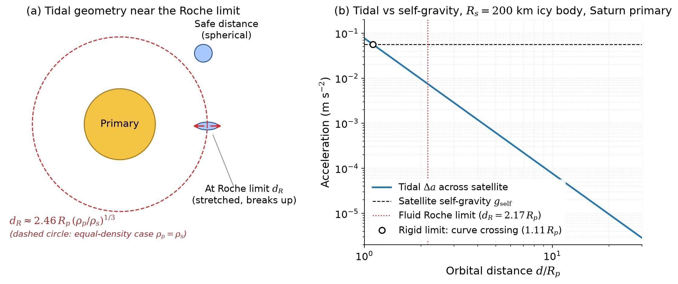
Fig. 2.20 Roche limit geometry. (a) A self-gravitating fluid satellite (blue) is rounded at safe orbital distance, but at the Roche limit \(d_R\) the differential tidal acceleration between its centre and its surface exceeds its self-gravity and it is stretched and torn apart along the line to the primary. (b) Tidal acceleration between the centre and the surface of a \(200\) km icy body compared with the body’s surface self-gravity, plotted against orbital distance from Saturn (in units of \(R_p\)). The simple crossing of the two curves defines the rigid Roche limit at \(d_R^{\mathrm{rigid}} \approx 1.11\,R_p\) for \(\rho_s = 1000\) kg m\(^{-3}\); the textbook fluid Roche limit \(d_R \approx 2.17\,R_p\) (red dotted line) carries an additional factor that accounts for tidal deformation of the satellite. Course-original figure.

Evaluating Eq. (2.6) for Saturn (\(R_p = 58{,}232\) km, \(\rho_p = 687\) kg m\(^{-3}\)) and an icy satellite (\(\rho_s \approx 1000\) kg m\(^{-3}\)):

\[ d_R \approx 2.46 \times 58{,}232 \times \left(\frac{687}{1000}\right)^{1/3} \approx 126{,}000 \text{ km} \approx 2.17\, R_p \]

Saturn’s main ring system (Fig. 2.21), the D through A rings, extends from about 67,000 km to 137,000 km from Saturn’s centre; the narrow F ring lies just beyond, at \(\sim 140{,}000\) km. The dense B and C rings sit well inside this fluid Roche limit, while much of the A ring’s radial extent lies beyond the nominal boundary: its sharp outer edge is maintained by a 7:6 mean-motion resonance with the moon Janus, and the ring particles are porous, so their density is below that of solid ice, which shifts the effective Roche limit outward. The rings consist of countless small particles that cannot coalesce into a moon because tidal forces prevent their gravitational aggregation. We will derive the Roche limit in full in Lecture 11.

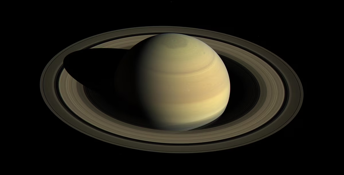
Fig. 2.21 Saturn and its rings imaged by the Cassini wide-angle camera in April 2016. The main ring system spans roughly \(67{,}000\) km to \(137{,}000\) km from Saturn’s centre, with the dense B and C rings well inside the fluid Roche limit at \(\sim 126{,}000\) km and much of the A ring’s width just outside it. The countless cm- to m-sized icy particles that make up the rings cannot coalesce into a moon because Saturn’s tides exceed their mutual self-gravity. Credit: NASA/JPL-Caltech/Space Science Institute (PIA21046).

2.9. Planetary migration

The orbits of planets are not fixed after formation. Interactions between planets and the disk (and later, between planets themselves) can cause substantial orbital migration, moving planets from their birth locations to very different orbits [Paardekooper et al., 2023].

2.9.1. Planet-disk interactions

A planet embedded in a gaseous disk excites spiral density waves at Lindblad resonances (the locations where the orbital frequency of the disk material differs from the planet’s by \(\pm \kappa/m\), with \(\kappa\) the local epicyclic frequency, the natural frequency of radial oscillations of a gas parcel, which equals the orbital frequency \(\Omega\) in a Keplerian disk, and \(m\) a positive integer, so that the planet’s periodic forcing resonates with the gas’s radial oscillations). These waves carry angular momentum away from the planet. Additionally, material co-orbiting with the planet (at the corotation resonances) exchanges angular momentum through horseshoe-shaped streamlines. The net torque on the planet determines whether it migrates inward or outward.

2.9.2. Types of migration

• Type I migration: A low-mass planet (below the gap-opening threshold, up to a few tens of Earth masses for typical disk parameters) remains fully embedded in the disk and migrates due to the imbalance between inner and outer Lindblad torques. In a simple disk model, the outer torque slightly dominates, driving inward migration on timescales of \(\sim 10^5\) years, potentially too fast, suggesting that additional physics (thermal effects, magnetic fields, disk structure) must slow or reverse migration in many cases.

• Type II migration: A massive planet (roughly Jupiter-mass and above) opens a gap in the disk, an annular region cleared of gas by the planet’s gravity. The planet then migrates on the slower viscous timescale of the disk (\(\sim 10^5\)–\(10^6\) years) as the disk accretes onto the star.

• Type III migration: In massive disks with a sharp density gradient near the planet, a rapid, runaway migration can occur when the co-orbital mass deficit (the difference between the disk mass that would fill the horseshoe region and the actual mass there) becomes comparable to the planet’s mass. This can cause very fast inward or outward migration.

The disk-flow patterns that drive these torques, including the spiral wakes at Lindblad resonances and the horseshoe streamlines at corotation, are shown in Fig. 2.22.

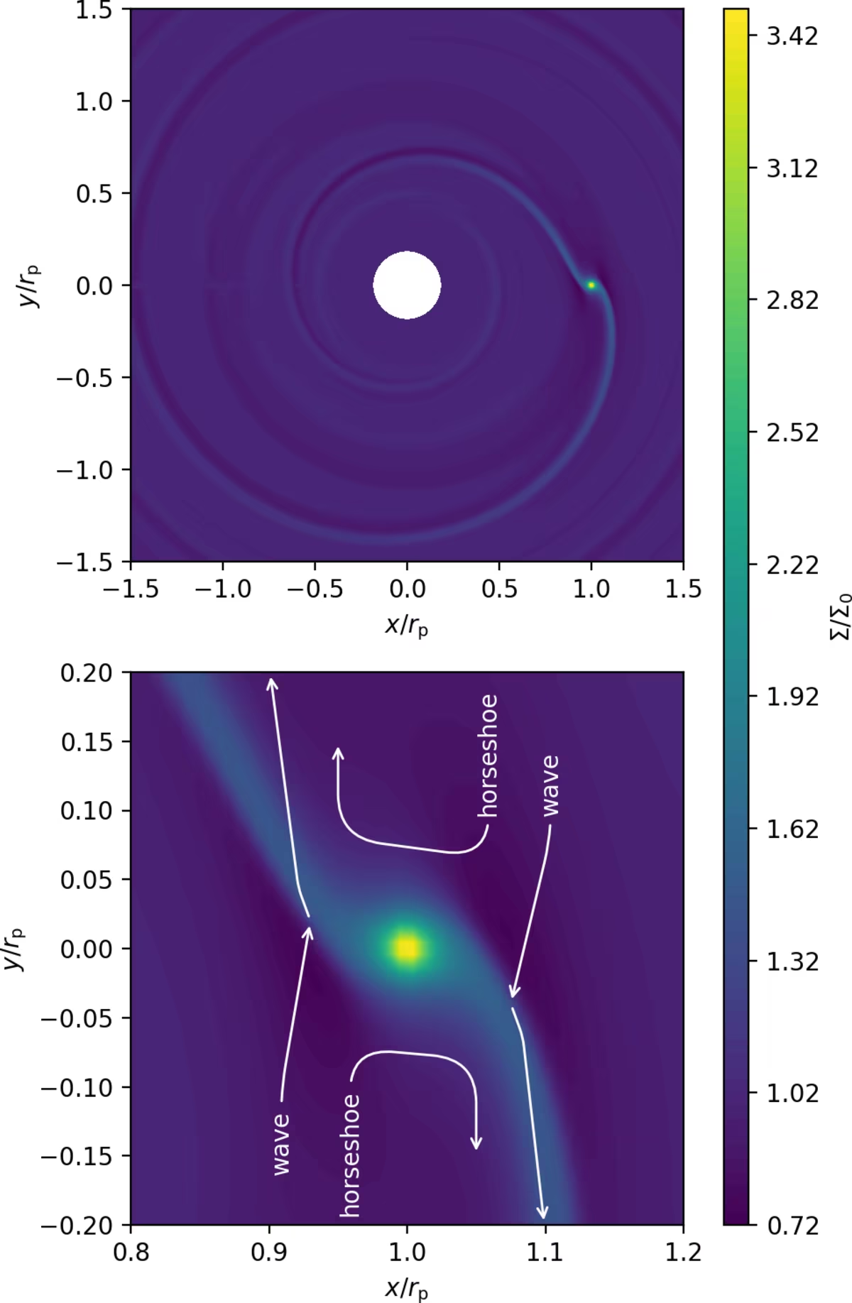
Fig. 2.22 Disk surface-density response to an embedded Neptune-mass planet (\(q = 10^{-4}\)) on a circular orbit. Top panel: the planet launches a one-armed spiral density wave; the colour scale gives the surface density relative to its unperturbed value (no gap is cleared at this planet mass). Bottom panel: zoom on the co-orbital region, with schematic streamlines marking the horseshoe trajectories and the trajectories feeding the spiral wave. The imbalance between the inner and outer wave torques, together with the corotation torque from the horseshoe region, sets the direction and speed of Type I migration. Adapted from Paardekooper et al. [2023], Fig. 2.

2.9.3. The Nice model

After the gas disk has dispersed, the giant planets can still undergo migration through interactions with a remnant disk of planetesimals. The Nice model [Tsiganis et al., 2005] proposes that the giant planets formed in a more compact configuration than today, with the outermost ice giant well inside Neptune’s present 30 AU orbit, and subsequently underwent a dynamical instability. In the original version of the model, the instability was triggered when Jupiter and Saturn slowly crossed their mutual 2:1 mean-motion resonance. Modern versions revise this picture: the orbital structure of the asteroid belt and the near-circular orbits of the terrestrial planets require that the Jupiter-Saturn period ratio changed discontinuously rather than smoothly, which is most naturally achieved if the outer solar system originally contained a fifth giant planet that was scattered off Jupiter and ejected during the instability, the so-called jumping-Jupiter scenario (Fig. 2.23) [Nesvorný, 2018]. In either version, the instability scattered Uranus and Neptune outward to their current orbits, disrupted the primordial Kuiper Belt, and delivered impactors throughout the inner solar system. An impact spike near 3.9 Gyr ago (the “Late Heavy Bombardment”) was long attributed to this instability, but the lunar evidence for the spike is now discounted: the impact ages cluster near 3.9 Gyr because every Apollo landing site samples ejecta of the Imbrium basin, and a smoothly declining impact flux fits the record equally well [Boehnke and Harrison, 2016]. Dynamical constraints instead favour an instability within the first \(\sim\)100 Myr after gas-disk dispersal [Nesvorný, 2018].

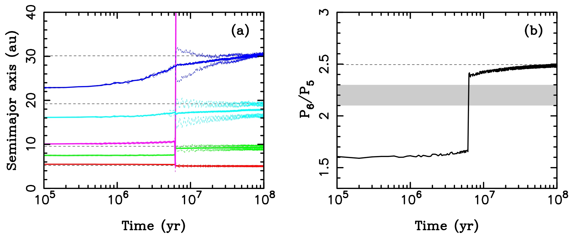
Fig. 2.23 Evolution of the giant planets through the Nice-model instability in a five-planet “jumping-Jupiter” simulation by Nesvorný and Morbidelli [2012]. Panel (a): semi-major axes vs time (solid lines) for five giant planets started in a compact resonant chain, with a fifth ice giant (magenta) initially between Saturn and Uranus; the dashed line of each colour pair is that planet’s perihelion and aphelion distance, so the width between them measures its eccentricity, and the horizontal grey dashed lines mark the present-day semi-major axes of the four surviving giants. At the instability (\(\sim 6\) Myr into this run) the extra ice giant is scattered off Jupiter and ejected from the solar system, while Uranus and Neptune move outward onto their present orbits. Panel (b): the Saturn/Jupiter period ratio, which begins near 1.6 in the initial resonant chain, first drifts slowly upward through planetesimal-driven migration and then jumps discontinuously (from \(\approx 1.7\) to \(\approx 2.4\) in under \(10^5\) yr) during the planet-planet encounters, approaching the present-day value of 2.49 (dashed line). The jump takes the system across the shaded band (\(2.1 \lesssim P_{\mathrm{Sat}}/P_{\mathrm{Jup}} \lesssim 2.3\)) in which slow migration would activate secular resonances (resonances between the slow precession rates of orbits, rather than between orbital periods) that excite the asteroid belt and the terrestrial-planet orbits; avoiding this zone is the central argument for the jumping-Jupiter scenario over the smooth 2:1 resonance crossing of the original Nice model [Tsiganis et al., 2005]. Reproduced from Nesvorný [2018], Fig. 3.

2.9.4. The Grand Tack

The Grand Tack hypothesis [Walsh et al., 2011] proposes that Jupiter first migrated inward to \(\sim 1.5\) AU via Type II migration, then reversed course when Saturn caught up and became trapped in the 3:2 mean-motion resonance with Jupiter: the combined torques from their mutual interaction with the disk drove both planets outward (“tacking,” as in sailing). This inward-then-outward migration (Fig. 2.24) would have scattered and depleted material in the inner solar system, potentially explaining the small mass of Mars and the compositional structure of the asteroid belt.

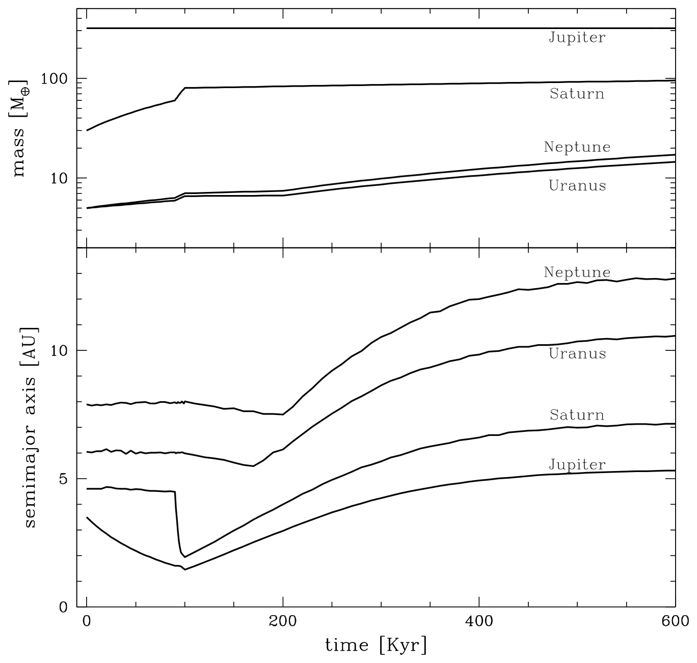
Fig. 2.24 The Grand Tack scenario. Top panel: the mass of each giant planet, with Jupiter fully formed from the start. Saturn’s core begins at \(30\,M_{\oplus}\) and reaches \(60\,M_{\oplus}\) over the first \(10^5\) yr, at which point its own inward migration begins; the cores of Uranus and Neptune grow from \(5\,M_{\oplus}\), and all three reach their full mass only at the end of the migration. Bottom panel: semi-major-axis evolution, with each curve labelled with the planet’s name; the tracks show the migration prescription imposed on the planets in the reference simulation, following the inward-then-outward path found in hydrodynamical studies. Jupiter migrates in to \(\sim 1.5\) AU; once Saturn catches up and the two planets become trapped in their mutual 3:2 mean-motion resonance, the migration reverses and both move outward. The episode depletes solid material in the inner disk, with consequences for Mars’s small mass and the asteroid belt’s compositional structure. Reproduced from Walsh et al. [2011], Fig. 1.

2.9.5. Observational evidence for migration

The strongest evidence that migration is real comes from hot Jupiters: gas giant exoplanets orbiting their host stars with periods of just a few days (\(a \lesssim 0.1\) AU). These planets cannot have formed in situ (there is not enough material, and temperatures are too high for solids to exist), so they must have formed further out and moved inward, either by disk migration or by later high-eccentricity migration followed by tidal circularisation (Fig. 2.25; Lecture 13). Additionally, ALMA observations of gaps in protoplanetary disks (such as those in HL Tau) may represent the signatures of embedded planets undergoing migration. We will revisit exoplanet demographics and the evidence for migration in Lecture 13.

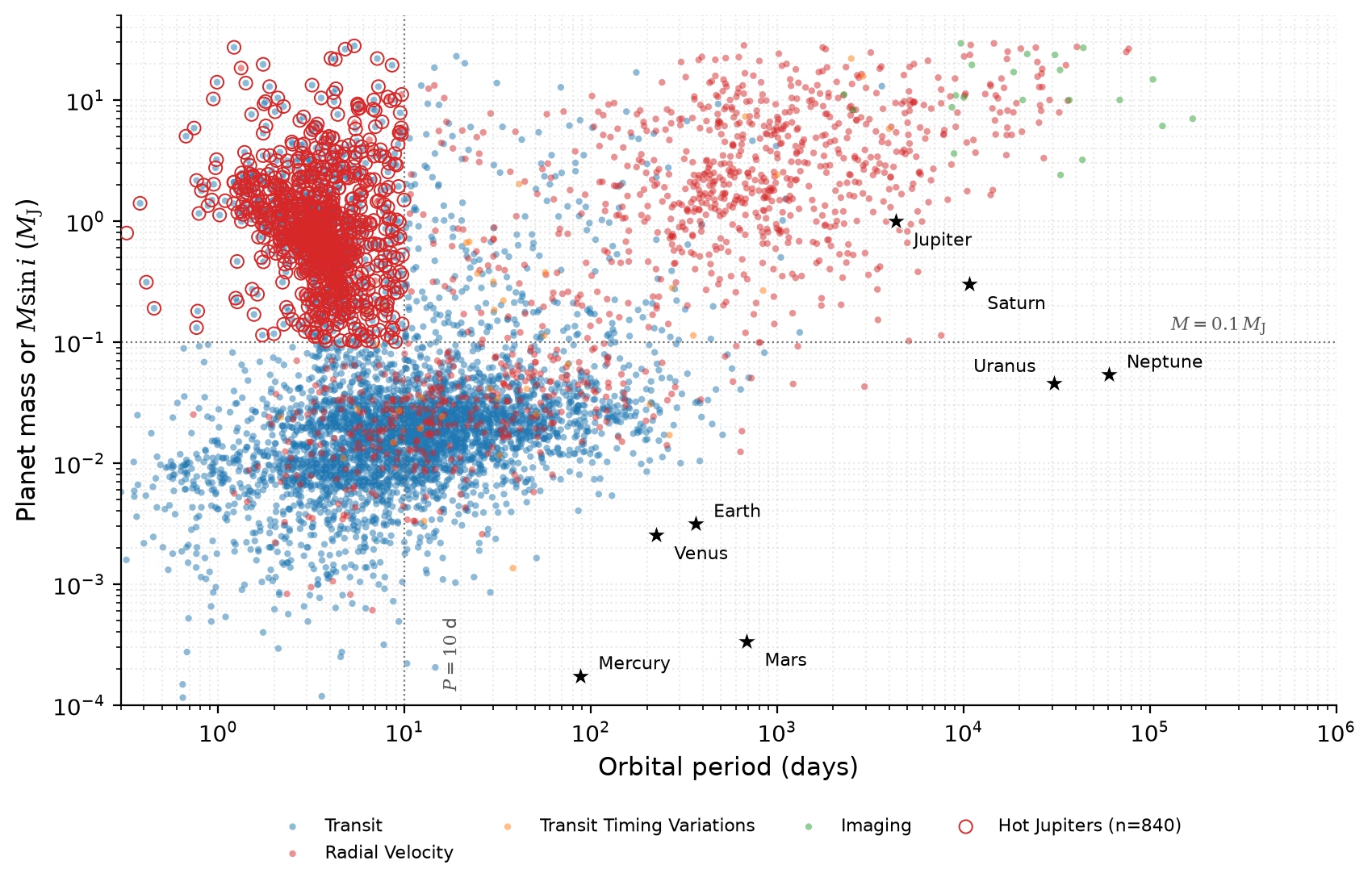
Fig. 2.25 Confirmed exoplanets in mass-period space, generated from the NASA Exoplanet Archive [NASA Exoplanet Archive, 2026] (accessed 2026-08). Detection methods are colour-coded, and the eight Solar System planets are overplotted as black stars for reference. Red circles mark the hot Jupiters, selected here as \(M > 0.1\,M_{\mathrm{J}}\) and \(P < 10\) d (dotted lines). This population cannot have formed in situ at such close-in orbital distances and is widely interpreted as evidence for large-scale orbital migration; see Dawson and Johnson [2018] for a review of the proposed pathways. Course-original figure.

2.10. Recent advances

The study of planet formation has been transformed by high-resolution imaging of protoplanetary disks. The ALMA DSHARP survey [Andrews et al., 2018] revealed rings and gaps in all 20 of its large, bright target disks, even around young (\(\lesssim 1\) Myr) stars. These structures are widely interpreted as signatures of embedded planets clearing gaps in the disk, although ice lines and magnetically structured zones remain viable alternatives for some of them; if planets are indeed responsible, planet formation begins earlier and proceeds faster than previously thought, consistent with the pebble-accretion paradigm [Lambrechts and Johansen, 2012].

Theoretical advances have been consolidated in the Protostars and Planets VII review volume [Drążkowska et al., 2023], which presents an updated synthesis of planet formation theory incorporating ALMA constraints. Key developments include refined models of the streaming instability that forms planetesimals, improved treatments of pebble accretion in evolving disks, new constraints on giant-planet formation timescales from isotopic analyses of meteorites [Kruijer et al., 2017], and the discovery of Jupiter’s dilute core in Juno gravity data [Wahl et al., 2017] (Lecture 8). Together these suggest that giant-planet cores grow within the first few Myr of disk evolution, before the gas disperses, although how early Jupiter’s core in particular had to form is still contested (Lecture 12, Lecture 14).

2.11. Looking ahead to Lecture 3

This lecture assembled the planets and set their orbits; the next asks what happens inside them. Lecture 3 follows the energy: the heat delivered by accretion and differentiation, the short-lived radionuclides (led by \(^{26}\mathrm{Al}\), half-life 0.72 Myr) that melted even small planetesimals, the long-lived isotopes that still power Earth’s 47 TW heat flow today, and the tidal dissipation whose consequences we just saw on Io. It then turns to how that heat escapes, by conduction and by convection, because the balance between the two decides whether a planet convects, sustains a dynamo, and stays geologically alive.

2.12. References

[Andrews2020] (1,2)

Andrews, Sean M. 2020. “Observations of protoplanetary disk structures.” Annual Review of Astronomy and Astrophysics, 58:483–528. doi:10.1146/annurev-astro-031220-010302, arXiv:2001.05007, https://ui.adsabs.harvard.edu/abs/2020ARA%26A..58..483A/abstract.

[Andrews2018] (1,2,3)

Andrews, Sean M., Huang, Jane, Pérez, Laura M., Isella, Andrea, Dullemond, Cornelis P., Kurtovic, Nicolás T., Guzmán, Viviana V., Carpenter, John M., Wilner, David J., Zhang, Shangjia, Zhu, Zhaohuan, Birnstiel, Til, Bai, Xue-Ning, Benisty, Myriam, Hughes, A. Meredith, Öberg, Karin I., and Ricci, Luca. 2018. “The disk substructures at high angular resolution project (DSHARP). I. Motivation, Sample, Calibration, and Overview.” The Astrophysical Journal Letters, 869(2):L41. doi:10.3847/2041-8213/aaf741, https://ui.adsabs.harvard.edu/abs/2018ApJ...869L..41A/abstract.

[Birnstiel2016] (1,2)

Birnstiel, Tilman, Fang, Min, and Johansen, Anders. 2016. “Dust evolution and the formation of planetesimals.” Space Science Reviews, 205(1-4):41–75. doi:10.1007/s11214-016-0256-1, arXiv:1604.05726, https://ui.adsabs.harvard.edu/abs/2016SSRv..205...41B/abstract.

[Blum2008] (1,2)

Blum, Jürgen and Wurm, Gerhard. 2008. “The growth mechanisms of macroscopic bodies in protoplanetary disks.” Annual Review of Astronomy and Astrophysics, 46:21–56. doi:10.1146/annurev.astro.46.060407.145152, https://ui.adsabs.harvard.edu/abs/2008ARA&A..46...21B/abstract.

[Boehnke2016]

Boehnke, Patrick and Harrison, T. Mark. 2016. “Illusory late heavy bombardments.” Proceedings of the National Academy of Sciences, 113(39):10802–10806. doi:10.1073/pnas.1611535113, https://ui.adsabs.harvard.edu/abs/2016PNAS..11310802B/abstract.

[Boss1997]

Boss, Alan P. 1997. “Giant planet formation by gravitational instability.” Science, 276(5320):1836–1839. doi:10.1126/science.276.5320.1836, https://ui.adsabs.harvard.edu/abs/1997Sci...276.1836B/abstract.

[DawsonJohnson2018]

Dawson, Rebekah I. and Johnson, John Asher. 2018. “Origins of hot jupiters.” Annual Review of Astronomy and Astrophysics, 56:175–221. doi:10.1146/annurev-astro-081817-051853, arXiv:1801.06117, https://ui.adsabs.harvard.edu/abs/2018ARA%26A..56..175D/abstract.

[Drazkowska2023] (1,2,3,4,5,6)

Drążkowska, Joanna, Bitsch, Bertram, Lambrechts, Michiel, Mulders, Gijs D., Harsono, Daniel, Vazan, Allona, Liu, Beibei, Ormel, Chris W., Kretke, Katherine, and Morbidelli, Alessandro. 2023. “Planet formation theory in the era of ALMA and Kepler: from pebbles to exoplanets.” In Inutsuka, Shu-ichiro, Aikawa, Yuri, Muto, Takayuki, Tomida, Kengo, and Tamura, Motohide, editors, Protostars and Planets VII. ASP Conference Series. doi:10.48550/arXiv.2203.09759, arXiv:2203.09759, https://ui.adsabs.harvard.edu/abs/2023ASPC..534..717D/abstract.

[Haisch2001]

Haisch, Jr., Karl E., Lada, Elizabeth A., and Lada, Charles J. 2001. “Disk frequencies and lifetimes in young clusters.” The Astrophysical Journal Letters, 553(2):L153–L156. doi:10.1086/320685, https://ui.adsabs.harvard.edu/abs/2001ApJ...553L.153H/abstract.

[Helled2014]

Helled, Ravit, Bodenheimer, Peter, Podolak, Morris, Boley, Aaron, Meru, Farzana, Nayakshin, Sergei, Fortney, Jonathan J., Mayer, Lucio, Alibert, Yann, and Boss, Alan P. 2014. “Giant planet formation, evolution, and internal structure.” In Beuther, Henrik, Klessen, Ralf S., Dullemond, Cornelis P., and Henning, Thomas, editors, Protostars and Planets VI, pages 643–665. University of Arizona Press. doi:10.2458/azu_uapress_9780816531240-ch028, arXiv:1311.1142, https://ui.adsabs.harvard.edu/abs/2014prpl.conf..643H/abstract.

[Johansen2007]

Johansen, Anders, Oishi, Jeffrey S., Mac Low, Mordecai-Mark, Klahr, Hubert, Henning, Thomas, and Youdin, Andrew. 2007. “Rapid planetesimal formation in turbulent circumstellar disks.” Nature, 448:1022–1025. doi:10.1038/nature06086, https://ui.adsabs.harvard.edu/abs/2007Natur.448.1022J/abstract.

[Kokubo1998] (1,2,3)

Kokubo, Eiichiro and Ida, Shigeru. 1998. “Oligarchic growth of protoplanets.” Icarus, 131(1):171–178. doi:10.1006/icar.1997.5840, https://ui.adsabs.harvard.edu/abs/1998Icar..131..171K/abstract.

[KratterLodato2016]

Kratter, Kaitlin M. and Lodato, Giuseppe. 2016. “Gravitational instabilities in circumstellar disks.” Annual Review of Astronomy and Astrophysics, 54:271–311. doi:10.1146/annurev-astro-081915-023307, arXiv:1603.01280, https://ui.adsabs.harvard.edu/abs/2016ARA%26A..54..271K/abstract.

[Krijt2023]

Krijt, Sebastiaan, Kama, Mihkel, McClure, Melissa, Teske, Johanna, Bergin, Edwin A., Shorttle, Oliver, Walsh, Kevin J., and Raymond, Sean N. 2023. “Chemical habitability: supply and retention of life's essential elements during planet formation.” In Inutsuka, Shu-ichiro, Aikawa, Yuri, Muto, Takayuki, Tomida, Kengo, and Tamura, Motohide, editors, Protostars and Planets VII. ASP Conference Series. doi:10.48550/arXiv.2203.10056, arXiv:2203.10056, https://ui.adsabs.harvard.edu/abs/2023ASPC..534.1031K/abstract.

[Kruijer2017]

Kruijer, Thomas S., Burkhardt, Christoph, Budde, Gerrit, and Kleine, Thorsten. 2017. “Age of Jupiter inferred from the distinct genetics and formation times of meteorites.” Proceedings of the National Academy of Sciences, 114(26):6712–6716. doi:10.1073/pnas.1704461114, https://ui.adsabs.harvard.edu/abs/2017PNAS..114.6712K/abstract.

[Lambrechts2012] (1,2,3)

Lambrechts, Michiel and Johansen, Anders. 2012. “Rapid growth of gas-giant cores by pebble accretion.” Astronomy & Astrophysics, 544:A32. doi:10.1051/0004-6361/201219127, https://ui.adsabs.harvard.edu/abs/2012A&A...544A..32L/abstract.

[Lichtenberg2021]

Lichtenberg, Tim, Drążkowska, Joanna, Schönbächler, Maria, Golabek, Gregor J., and Hands, Thomas O. 2021. “Bifurcation of planetary building blocks during Solar System formation.” Science, 371(6527):365–370. doi:10.1126/science.abb3091, arXiv:2101.08571, https://ui.adsabs.harvard.edu/abs/2021Sci...371..365L/abstract.

[Lichtenberg2023]

Lichtenberg, Tim, Schaefer, Laura K., Nakajima, Miki, and Fischer, Rebecca A. 2023. “Geophysical evolution during rocky planet formation.” In Inutsuka, Shu-ichiro, Aikawa, Yuri, Muto, Takayuki, Tomida, Kengo, and Tamura, Motohide, editors, Protostars and Planets VII. ASP Conference Series. doi:10.48550/arXiv.2203.10023, arXiv:2203.10023, https://ui.adsabs.harvard.edu/abs/2023ASPC..534..907L/abstract.

[Lissauer2009]

Lissauer, Jack J., Hubickyj, Olenka, D'Angelo, Gennaro, and Bodenheimer, Peter. 2009. “Models of Jupiter's growth incorporating thermal and hydrodynamic constraints.” Icarus, 199(2):338–350. doi:10.1016/j.icarus.2008.10.004, arXiv:0810.5186, https://ui.adsabs.harvard.edu/abs/2009Icar..199..338L/abstract.

[Miotello2023]

Miotello, Anna, Kamp, Inga, Birnstiel, Til, Cleeves, L. Ilsedore, and Kataoka, Akimasa. 2023. “Setting the stage for planet formation: measurements and implications of the fundamental disk properties.” In Inutsuka, Shu-ichiro, Aikawa, Yuri, Muto, Takayuki, Tomida, Kengo, and Tamura, Motohide, editors, Protostars and Planets VII. ASP Conference Series. doi:10.48550/arXiv.2203.09818, arXiv:2203.09818, https://ui.adsabs.harvard.edu/abs/2023ASPC..534..501M/abstract.

[MurrayDermott1999] (1,2,3)

Murray, Carl D. and Dermott, Stanley F. 1999. Solar System Dynamics. Cambridge University Press, Cambridge. doi:10.1017/CBO9781139174817, https://ui.adsabs.harvard.edu/abs/1999ssd..book.....M/abstract.

[Nesvorny2018] (1,2,3)

Nesvorný, David. 2018. “Dynamical evolution of the early solar system.” Annual Review of Astronomy and Astrophysics, 56:137–174. doi:10.1146/annurev-astro-081817-052028, arXiv:1807.06647, https://ui.adsabs.harvard.edu/abs/2018ARA%26A..56..137N/abstract.

[NesvornyMorbidelli2012]

Nesvorný, David and Morbidelli, Alessandro. 2012. “Statistical study of the early Solar System's instability with four, five, and six giant planets.” The Astronomical Journal, 144(4):117. doi:10.1088/0004-6256/144/4/117, arXiv:1208.2957, https://ui.adsabs.harvard.edu/abs/2012AJ....144..117N/abstract.

[Paardekooper2023] (1,2)

Paardekooper, Sijme-Jan, Dong, Ruobing, Duffell, Paul, Fung, Jeffrey, Masset, Frédéric, Ogilvie, Gordon, and Tanaka, Hidekazu. 2023. “Planet–disk interactions and orbital evolution.” In Inutsuka, Shu-ichiro, Aikawa, Yuri, Muto, Takayuki, Tomida, Kengo, and Tamura, Motohide, editors, Protostars and Planets VII. ASP Conference Series. doi:10.48550/arXiv.2203.09595, arXiv:2203.09595, https://ui.adsabs.harvard.edu/abs/2023ASPC..534..685P/abstract.

[Peale1979] (1,2)

Peale, Stanton J., Cassen, Patrick, and Reynolds, Ray T. 1979. “Melting of Io by tidal dissipation.” Science, 203(4383):892–894. doi:10.1126/science.203.4383.892, https://ui.adsabs.harvard.edu/abs/1979Sci...203..892P/abstract.

[Pollack1996] (1,2)

Pollack, James B., Hubickyj, Olenka, Bodenheimer, Peter, Lissauer, Jack J., Podolak, Morris, and Greenzweig, Yuval. 1996. “Formation of the giant planets by concurrent accretion of solids and gas.” Icarus, 124(1):62–85. doi:10.1006/icar.1996.0190, https://ui.adsabs.harvard.edu/abs/1996Icar..124...62P/abstract.

[Simon2016] (1,2)

Simon, Jacob B., Armitage, Philip J., Li, Rixin, and Youdin, Andrew N. 2016. “The mass and size distribution of planetesimals formed by the streaming instability. I. the role of self-gravity.” The Astrophysical Journal, 822(1):55. doi:10.3847/0004-637X/822/1/55, arXiv:1512.00009, https://ui.adsabs.harvard.edu/abs/2016ApJ...822...55S/abstract.

[Tsiganis2005] (1,2)

Tsiganis, Kleomenis, Gomes, Rodney, Morbidelli, Alessandro, and Levison, Harold F. 2005. “Origin of the orbital architecture of the giant planets of the Solar System.” Nature, 435:459–461. doi:10.1038/nature03539, https://ui.adsabs.harvard.edu/abs/2005Natur.435..459T/abstract.

[Wahl2017]

Wahl, Sean M., Hubbard, William B., Militzer, Burkhard, Guillot, Tristan, Miguel, Yamila, Movshovitz, Nadine, Kaspi, Yohai, Helled, Ravit, Reese, David, Galanti, Eli, Levin, Steve, Connerney, John E. P., and Bolton, Scott J. 2017. “Comparing Jupiter interior structure models to Juno gravity measurements and the role of a dilute core.” Geophysical Research Letters, 44(10):4649–4659. doi:10.1002/2017GL073160, arXiv:1707.01997, https://ui.adsabs.harvard.edu/abs/2017GeoRL..44.4649W/abstract.

[Walsh2011] (1,2)

Walsh, Kevin J., Morbidelli, Alessandro, Raymond, Sean N., O'Brien, David P., and Mandell, Avi M. 2011. “A low mass for Mars from Jupiter's early gas-driven migration.” Nature, 475:206–209. doi:10.1038/nature10201, https://ui.adsabs.harvard.edu/abs/2011Natur.475..206W/abstract.

[NSSDCPlanetaryFactSheet]

Williams, David R. 2026. Planetary fact sheet. NASA Goddard Space Flight Center, NSSDCA. Accessed 2026-08-08. https://nssdc.gsfc.nasa.gov/planetary/factsheet/.

[WilliamsCieza2011]

Williams, Jonathan P. and Cieza, Lucas A. 2011. “Protoplanetary disks and their evolution.” Annual Review of Astronomy and Astrophysics, 49:67–117. doi:10.1146/annurev-astro-081710-102548, arXiv:1103.0556, https://ui.adsabs.harvard.edu/abs/2011ARA%26A..49...67W/abstract.

[Oberg2011]

Öberg, Karin I., Murray-Clay, Ruth, and Bergin, Edwin A. 2011. “The effects of snowlines on C/O in planetary atmospheres.” The Astrophysical Journal Letters, 743(1):L16. doi:10.1088/2041-8205/743/1/L16, arXiv:1110.5567, https://ui.adsabs.harvard.edu/abs/2011ApJ...743L..16O/abstract.

[ALMAPartnership2015] (1,2)

ALMA Partnership, Brogan, C. L., Pérez, L. M., Hunter, T. R., Dent, W. R. F., Hales, A. S., Hills, R. E., Corder, S., Fomalont, E. B., Vlahakis, C., and others. 2015. “The 2014 ALMA long baseline campaign: first results from high angular resolution observations toward the HL Tau region.” The Astrophysical Journal Letters, 808(1):L3. doi:10.1088/2041-8205/808/1/L3, https://ui.adsabs.harvard.edu/abs/2015ApJ...808L...3A/abstract.

[NASAExoplanetArchive2026]

NASA Exoplanet Archive. 2026. NASA Exoplanet Archive: Confirmed Planets Table. NASA Exoplanet Science Institute, Caltech/IPAC. Accessed 2026-04-16. doi:10.26133/NEA1, https://exoplanetarchive.ipac.caltech.edu/.