9. Rocky Planets, Earth & Venus#
Learning objectives: By the end of this lecture, you will be able to describe Earth’s unique properties as a reference planet, explain how Venus diverged from Earth despite similar bulk composition and size, apply the Simpson-Nakajima runaway greenhouse limit, and evaluate the role of water loss history, tectonic regime, and the carbonate-silicate cycle in comparative habitability.
See also
Slides: Download Lecture 9 (PDF)
Earth and Venus are nature’s best controlled experiment in comparative planetology. They formed from the same nebular reservoir within roughly \(0.3\) AU of each other (Fig. 9.1), contain similar bulk inventories of silicate, iron, and volatile elements, and have masses and radii within \(20\%\) of each other. Yet their present-day surface conditions could not be more different. Earth is wet, geologically active, magnetically shielded, and inhabited. Venus is dry, encased in a \(92\) bar carbon-dioxide atmosphere at a surface temperature of \(737\) K, and the only one of the rocky planets without a global magnetic field. Identifying what set these two nearly identical starting points on such radically different evolutionary paths is the central question of this lecture. This lecture works through that question in three parts. Part 1 reviews Earth as a reference planet, Part 2 surveys Venus as the alien twin, and Part 3 brings the comparison together to extract the underlying physics. The blackboard derivation in the middle introduces the Simpson-Nakajima runaway greenhouse limit, a thermodynamic boundary in phase space that, once crossed, makes the divergence essentially irreversible.
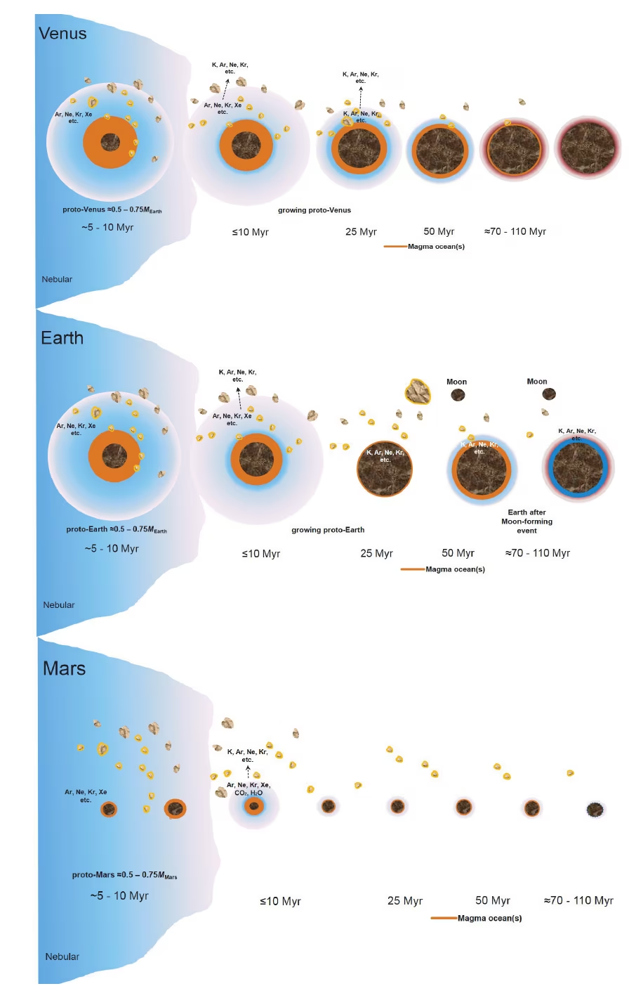
Fig. 9.1 Schematic accretion histories of Venus (top), Earth (middle), and Mars (bottom) during the first \(\sim\)110 Myr of the Solar System. Each panel sketches the buildup from undifferentiated planetesimals through differentiated planetary embryos to the final magma-ocean stage, in which intense early heating leaves the planet’s outer layers wholly or partly molten. Volatile species (\(\mathrm{H_2O}\), \(\mathrm{CO_2}\), noble gases) outgas from the interior to form a primary steam-rich atmosphere; their fate during the cooling of the magma ocean determines the long-term volatile inventory of each planet. Reproduced from Lammer et al. [2018].#
9.1. Part 1: Earth as reference#
9.1.1. Earth’s bulk properties and what makes it habitable#
Earth has a semimajor axis of \(1\) AU, mass \(\Mearth = 5.97 \times 10^{24}\) kg, and equatorial radius \(\Rearth = 6378\) km. Its mean density of \(5.51\) g/cm\(^3\), the highest in the Solar System, indicates a differentiated interior with a metallic iron-nickel core (Lecture 8) [Dziewonski and Anderson, 1981]. The dimensionless moment of inertia factor is \(C/MR^2 = 0.331\), compared to \(0.4\) for a uniform sphere. This indicates that an iron core holds \(32\%\) of Earth’s mass in \(17\%\) of its volume. Mean surface conditions are \(T_s \approx 288\) K and \(P_s = 1.013\) bar, under an atmosphere of \(78\%\) \(\mathrm{N_2}\), \(21\%\) \(\mathrm{O_2}\), and trace species (argon, water vapour, \(\mathrm{CO_2}\)).
Earth is unique today in combining three coupled systems: an active mobile-lid plate tectonic regime, where the rigid outer shell is broken into independently moving plates; persistent liquid surface water covering \(71\%\) of the planet; and a global biosphere. Liquid water hydrates the lithosphere, the rigid outer shell comprising the crust and uppermost mantle. This enables subduction, the sinking of one plate beneath another into the mantle (Lecture 7). Persistent liquid water on \(4\)-Gyr timescales is stabilised by the carbonate-silicate cycle (Lecture 6), a negative feedback requiring volcanic outgassing of \(\mathrm{CO_2}\) and silicate weathering on a wet surface [Walker et al., 1981]. The biosphere acts on top of this abiotic feedback and has set the atmospheric \(\mathrm{O_2}\) level for the last \(\sim\)2.4 billion years [Lyons et al., 2014]. This mutual coupling maintains Earth’s habitability over billions of years, supporting the coexisting oceans, atmosphere, and ice sheets visible from space (Fig. 9.2). Removing any component causes the system to collapse, as likely occurred early on Venus.
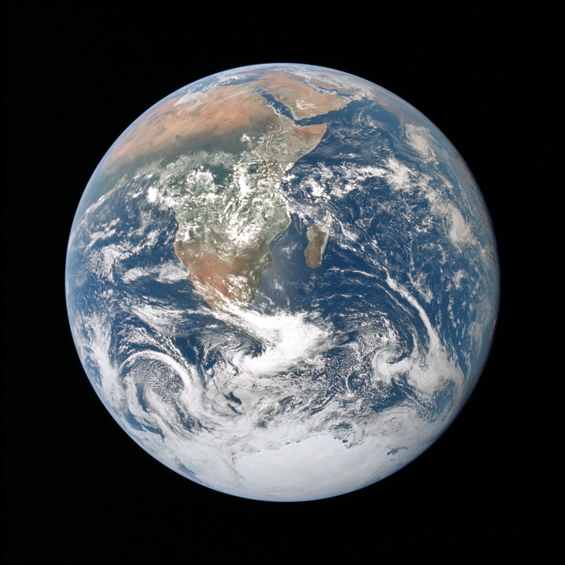
Fig. 9.2 “The Blue Marble”, Apollo 17, 7 December 1972. Earth photographed by the crew en route to the Moon, with the hydrosphere and cryosphere visible together. Ocean covers most of the sunlit disk on both sides of Africa, from the South Atlantic in the west to the Indian Ocean in the east, while the Antarctic ice cap forms the bright cryosphere along the lower limb. Africa, the Arabian Peninsula, and Madagascar lie near the centre of the disk. NASA image AS17-148-22727. Credit: NASA / Apollo 17 crew.#
9.1.2. The geologic eons of Earth#
Geologists divide the \(4.54\) Gyr of Earth history into four eons, the primary formal subdivisions of geologic time (Fig. 9.3). Boundary ages are calibrated by radiometric dating (Lecture 12) and standardised in the Geologic Time Scale [Gradstein et al., 2020].
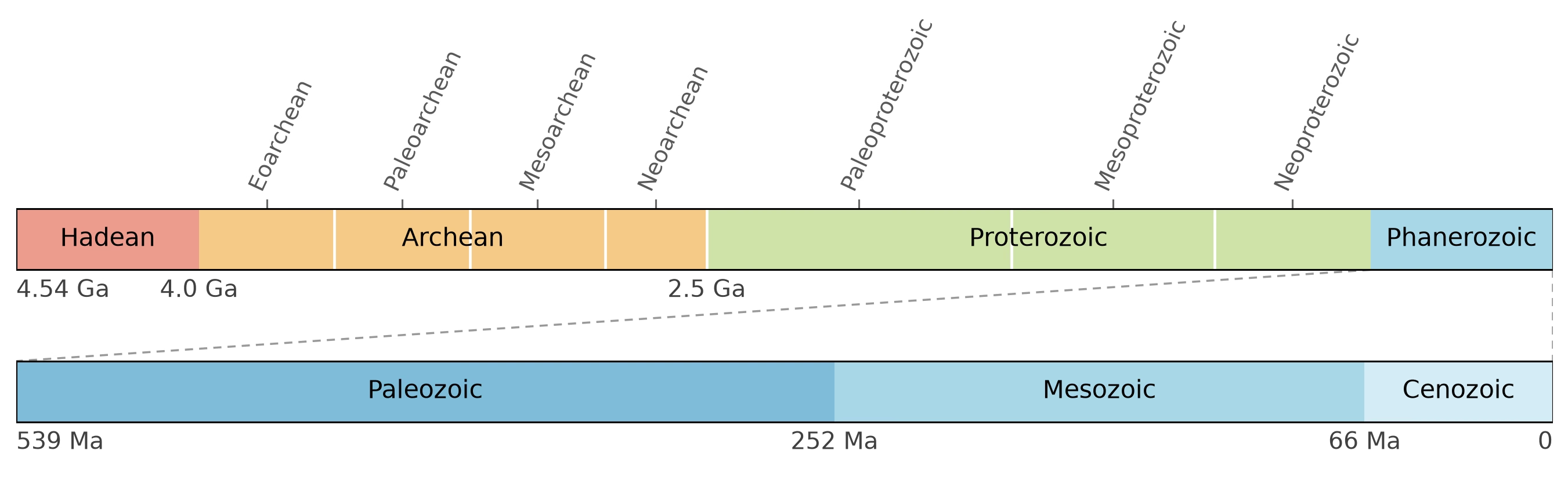
Fig. 9.3 The geologic eons and eras of Earth. Top bar: the four eons spanning the full \(4.54\) Gyr of Earth history, with the eras of the Archean and Proterozoic marked above; note that the Hadean, Archean, and Proterozoic together (the informal “Precambrian”) occupy almost \(90\%\) of the timeline. Bottom bar: the Phanerozoic eon stretched to the full figure width, divided into the Paleozoic, Mesozoic, and Cenozoic eras at the end-Permian (\(252\) Ma) and end-Cretaceous (\(66\) Ma) mass extinctions. Boundary ages follow the Geologic Time Scale 2020 [Gradstein et al., 2020].#
The Hadean eon (\(4.54\) to \(4.0\) Ga) covers accretion, the Moon-forming impact (Lecture 4), magma ocean solidification, and early crust and oceans. Detrital zircons from Jack Hills date to \(4.4\) Ga, with oxygen isotopes indicating liquid surface water and continental crust formed within \(\sim\)150 Myr of formation [Wilde et al., 2001].
The Archean eon (\(4.0\) to \(2.5\) Ga) preserves the oldest continental rocks (\(4.0\) Gyr), an active geodynamo by \(3.45\) Ga [Tarduno et al., 2010], early life, and an anoxic \(\mathrm{N_2}\) and \(\mathrm{CO_2}\) atmosphere with methane [Catling and Zahnle, 2020]. The Proterozoic eon (\(2.5\) Ga to \(539\) Ma) spans from the Great Oxidation Event and Huronian glaciations (\(\sim\)2.4 Ga) to Neoproterozoic Snowball Earth episodes and the first macroscopic animals. The Phanerozoic eon (\(539\) Ma to present, meaning “visible life”) encompasses animal and plant evolution, punctuated by mass extinctions at \(252\) Ma and \(66\) Ma, the latter from the Chicxulub impact (Lecture 12). Precambrian milestones provide the foundation for habitability (Lecture 13, Lecture 14).
9.1.3. Plate tectonics in action#
Subduction is the return leg of the carbon cycle (Lecture 7). Volcanic \(\mathrm{CO_2}\) reacts with silicate minerals in the presence of liquid water to form carbonate sediments, which are subducted into the mantle and partly recycled to the atmosphere [Krissansen-Totton et al., 2018]. This cycle equilibrates atmospheric \(\mathrm{CO_2}\) on a timescale of \(\sim\)0.5 Myr [Walker et al., 1981]. Without subduction, carbon released from the interior accumulates in the atmosphere indefinitely, as on Venus (Fig. 9.4).
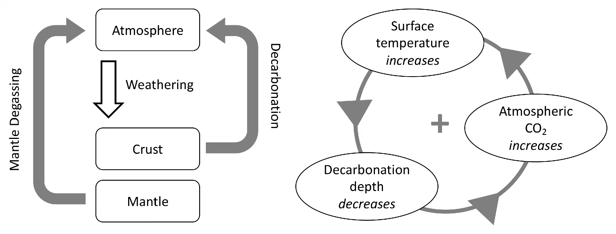
Fig. 9.4 Schematic of the carbon cycle on a stagnant-lid Venus, a planet whose rigid outer shell forms a single immobile plate rather than being broken into moving tectonic plates, from Höning et al. [2021]. Left: the three carbon reservoirs (mantle, crust, atmosphere) are coupled by mantle degassing (volcanism), surface weathering of fresh basaltic crust, and decarbonation of buried carbonate when the crust heats up. Right: the destabilising positive feedback loop. Increasing surface temperature shifts the geotherm (the profile of temperature with depth) upward, which pushes the decarbonation isotherm to shallower depth in the crust, releasing buried \(\mathrm{CO_2}\) to the atmosphere and raising the surface temperature further. Without subduction, there is no return leg to the mantle to break the loop. Reproduced from Höning et al. [2021].#
9.1.4. Earth’s magnetic field and its consequences#
Earth possesses a global magnetic field driven by the geodynamo (Lecture 4). Surface field strengths are \(25\) to \(65\) microtesla. Palaeomagnetic measurements of single zircon crystals show that this dynamo has operated for at least \(3.45\) Gyr [Tarduno et al., 2010].
The resulting magnetosphere (Fig. 9.5) deflects the solar wind into a cavity extending roughly \(10\, \Rearth\) on the dayside. It shields the surface from ionising radiation. It suppresses atmospheric loss by eliminating ion-pickup escape, the acceleration of atmospheric ions by the solar-wind motional electric field across closed field lines. Earth still loses hydrogen through Jeans escape (thermal loss of high-velocity atoms) and polar wind (ion outflow along open magnetic field lines near the poles). These loss rates are far lower than the escape that desiccated Mars after its dynamo died around \(4.1\) to \(3.9\) Ga (Lecture 10) and stripped early Venus under solar EUV radiation [Lammer et al., 2018]. Venus lacks a detectable internal magnetic field today, a contrast explored in Part 2.
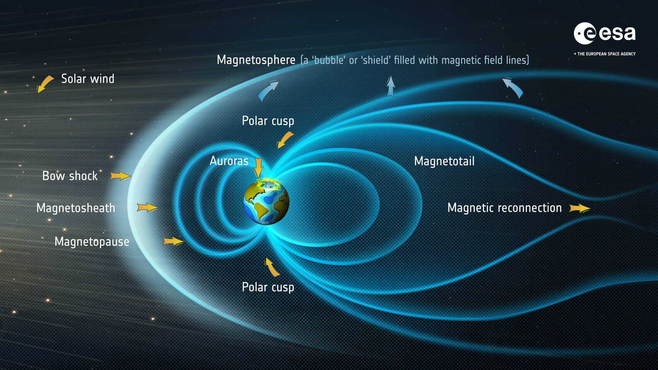
Fig. 9.5 Structure of Earth’s magnetosphere. The solar wind (orange arrows, arriving from the left) is deflected at the bow shock, and the shocked plasma flows around the planet through the magnetosheath. The magnetopause, where the solar-wind ram pressure balances the magnetic pressure of Earth’s field, stands at roughly \(10\,\Rearth\) on the dayside, while the nightside field is drawn out into the long magnetotail. This cavity shields the surface from most solar-wind particles and suppresses ion-pickup escape from the regions of closed field lines, in contrast to the open field lines at the poles that permit polar wind. Credit: ESA, CC BY-SA 3.0 IGO.#
9.1.5. The hydrosphere and cryosphere#
The oceans hold \(1.34 \times 10^{21}\) kg of water (about \(97\%\)). This is a \(2.7\) km global equivalent layer. The cryosphere (the frozen water reservoir) holds \(\sim\)2%, with remaining water contributing \(\sim\)1%.
The carbonate buffer balances dissolved \(\mathrm{CO_2}\), \(\mathrm{CO_3^{2-}}\), and \(\mathrm{HCO_3^-}\). Ocean \(\mathrm{pH}\) stays near \(8.1\). This enables the carbonate-silicate cycle (Fig. 9.6), whose sink is the Urey reaction (Lecture 6):
Silicate rock weathered by dissolved \(\mathrm{CO_2}\) yields carbonate, which precipitates on the seafloor and removes the carbon from the atmosphere [Walker et al., 1981].
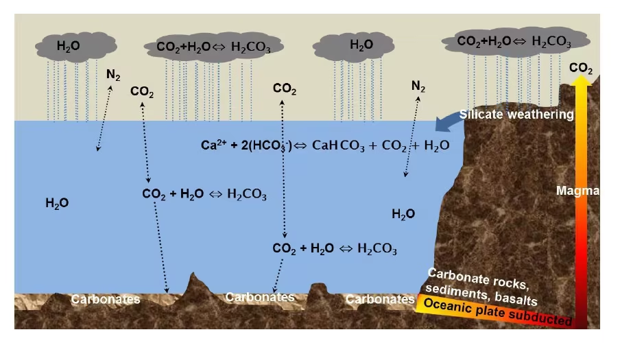
Fig. 9.6 Cartoon of the carbonate-silicate cycle on a planet with active plate tectonics. Atmospheric \(\mathrm{CO_2}\) dissolves in rainwater to form weak carbonic acid, which weathers continental silicates into bicarbonate ions; rivers transport these to the ocean, where they are precipitated as carbonate rocks; subduction then returns the carbon to the mantle. Volcanism completes the cycle by outgassing fresh \(\mathrm{CO_2}\). On geological timescales (of order \(0.5\) Myr), this cycle stabilises the surface temperature against perturbations. Reproduced from Lammer et al. [2018].#
9.1.6. Earth’s climate system#
Following Lecture 5 and Lecture 6, Earth absorbs \(240\) W/m\(^2\) of solar radiation (albedo \(\sim\)0.30) and emits equally in the infrared. Without an atmospheric greenhouse, the equilibrium temperature is \(255\) K. The natural greenhouse effect warms the surface by \(33\) K to \(288\) K. Water vapour contributes about half of this effect, clouds about a quarter, and \(\mathrm{CO_2}\) about a fifth [Schmidt et al., 2010].
The faint young Sun problem is the contradiction between a \(30\%\) fainter early Sun at \(4.4\) Ga and geological evidence for liquid water from at least \(4.3\) Ga [Feulner, 2012]. Higher early levels of \(\mathrm{CO_2}\), and possibly \(\mathrm{CH_4}\), most likely resolved this. Silicate weathering then drew them down as the Sun brightened (Fig. 9.7) (Fig. 9.8).
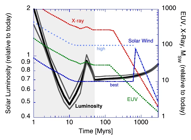
Fig. 9.7 Solar luminosity (left axis, solid black curve) and EUV/X-ray flux (right axis, coloured curves) over the first \(\sim\)5 Gyr after the Sun reached the main sequence, normalised to present values. The bolometric luminosity has risen by about \(30\%\) since \(4.5\) Ga, while the EUV and X-ray fluxes have dropped by factors of \(10\)–\(1000\) from the young, magnetically active Sun. The faint-young-Sun problem is the apparent contradiction between this lower bolometric flux and geological evidence for liquid water on early Earth. Reproduced from Zahnle et al. [2007].#
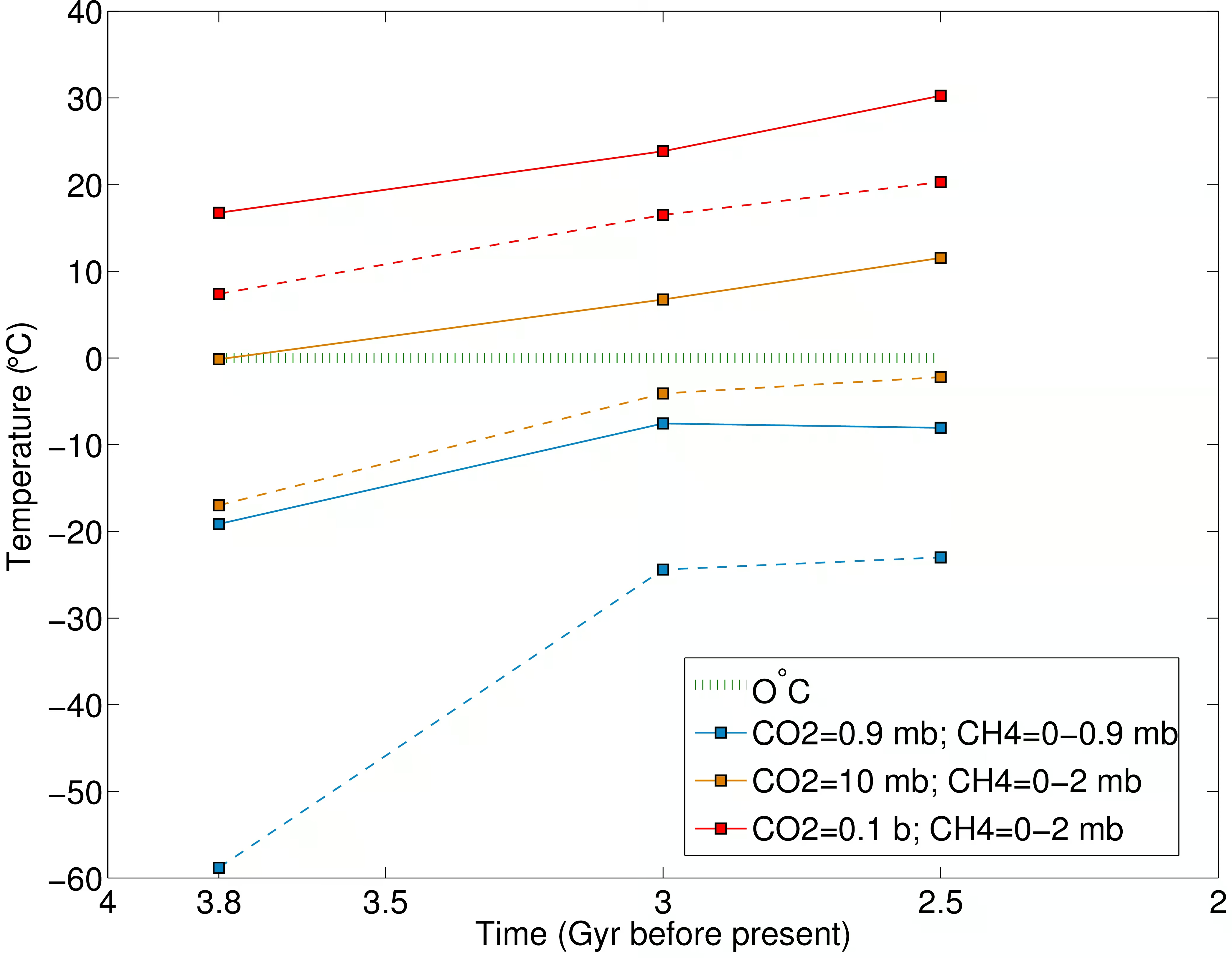
Fig. 9.8 Three-dimensional general-circulation model results for the global mean surface temperature of the Archean Earth between \(3.8\) Ga and \(2.5\) Ga, from Charnay et al. [2013]. Curves show solutions for three atmospheric compositions: \(0.9\) mbar \(\mathrm{CO_2}\) with \(0.9\) mbar \(\mathrm{CH_4}\) (blue), \(10\) mbar \(\mathrm{CO_2}\) with \(2\) mbar \(\mathrm{CH_4}\) (orange), and \(0.1\) bar \(\mathrm{CO_2}\) with \(2\) mbar \(\mathrm{CH_4}\) (red); solid lines include methane and dashed lines omit it. The dotted green line marks the freezing point of water. A few mbar of \(\mathrm{CO_2}\) together with trace methane is marginal at \(3.8\) Ga but warms by \(3\) Ga, while \(\sim\)0.1 bar of \(\mathrm{CO_2}\) together with trace methane comfortably resolves the faint-young-Sun problem at all three epochs. Reproduced from Charnay et al. [2013].#
9.1.7. Snowball Earth episodes#
During the Cryogenian period, Earth experienced global glaciations (Fig. 9.9) documented by the Sturtian (roughly \(717\) to \(660\) Ma) and Marinoan (\(645\) to \(635\) Ma) episodes [Hoffman et al., 2017]. Geological evidence includes glacial diamictites (poorly sorted glacial deposits) preserved within \(10^\circ\) of the equator. Banded iron formations returned after a billion-year absence. These glacial layers are capped by thick cap carbonates that record an abrupt transition to warm greenhouse conditions immediately after deglaciation.
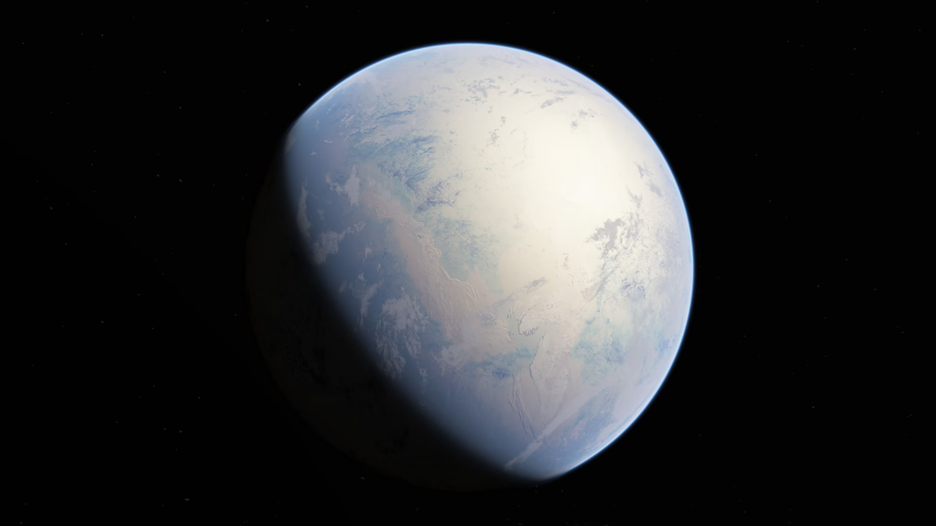
Fig. 9.9 Artist’s impression of a fully ice-covered “snowball” Earth, with the continents buried under ice and only faint outlines visible. The bright frozen surface reflects most of the incoming sunlight; this high albedo is what makes the snowball state self-sustaining until volcanic \(\mathrm{CO_2}\) accumulates enough to force deglaciation. Credit: Oleg Kuznetsov (3depix.com), Wikimedia Commons, CC BY-SA 4.0.#

These episodes demonstrate that the carbonate-silicate thermostat (the Walker feedback, Lecture 6) operates symmetrically to rescue the planet from extreme cold states as well as warm ones. While Venus failed by overheating, Earth nearly failed by freezing. That Earth survived both is a measure of how robust the carbonate-silicate feedback is, provided liquid water and active volcanism both persist.
9.1.8. Earth today in its long-term context#
Anthropogenic climate change is a planetary-scale perturbation governed by the same greenhouse physics as Venus.
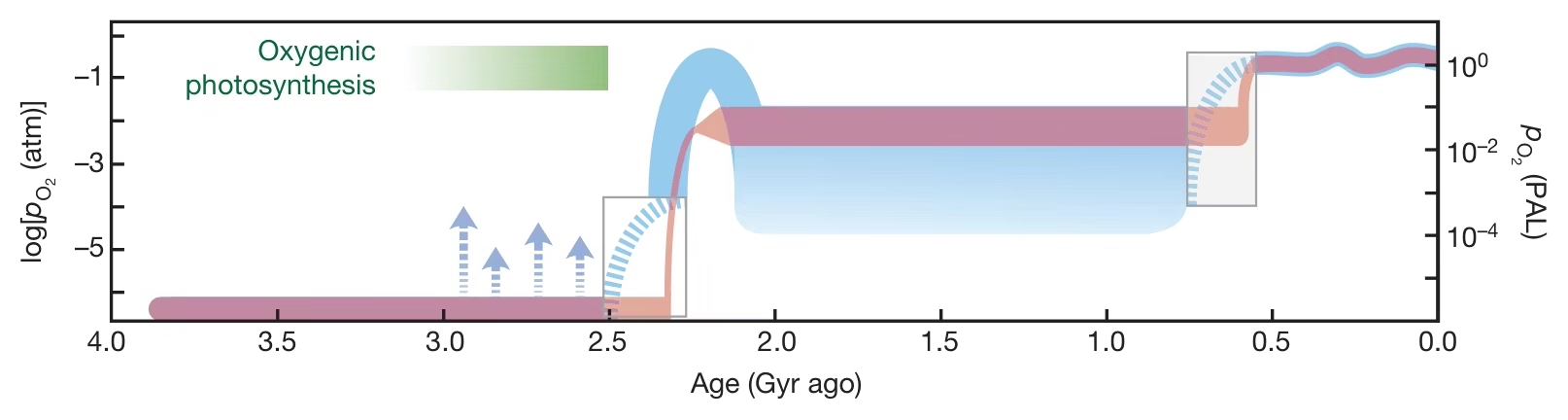
Fig. 9.10 Evolution of Earth’s atmospheric oxygen content through time, on a logarithmic scale of \(p\mathrm{O_2}\) relative to present atmospheric level (PAL). The atmosphere remained essentially anoxic (\(p\mathrm{O_2} < 10^{-5}\) PAL) for the first \(\sim\)2 Gyr of Earth history, then rose abruptly during the Great Oxidation Event at \(\sim\)2.4 Ga, plateaued at intermediate values through the mid-Proterozoic, and rose again to near-modern levels in the Neoproterozoic and Phanerozoic. The two-stage rise reflects the gradual buildup of the photosynthetic biosphere and shifting redox balance with the deep ocean and crust. Reproduced from Lyons et al. [2014].#
The carbonate-silicate thermostat cannot buffer climate on human timescales. Silicate weathering equilibrates \(\mathrm{CO_2}\) over \(\sim\)0.5 Myr, roughly five orders of magnitude slower than the perturbation. The radiative physics that warms Venus to \(737\) K operates on Earth. The \(4\)-Gyr geological feedbacks cannot compensate on human timescales.
9.1.9. The biosphere’s geological footprint#
The biosphere has rewritten Earth’s surface chemistry in ways that distinguish it from Venus. The Great Oxidation Event at \(\sim\)2.4 Ga marks the rise of atmospheric \(\mathrm{O_2}\) from negligible Archean levels (pre-GOE \(p_{\mathrm{O_2}} < 10^{-5}\) atm) to roughly \(0.1\text{--}1\%\) of modern values, driven by oxygenic photosynthesis by cyanobacteria [Lyons et al., 2014]. In the rock record, banded iron formations disappeared. Redbeds (sediments reddened by iron oxide in an oxidising environment) appeared. A second oxygenation step in the late Neoproterozoic raised \(\mathrm{O_2}\) to near-modern values just before the Cambrian explosion. Fig. 9.11 places these events on the Precambrian time scale.
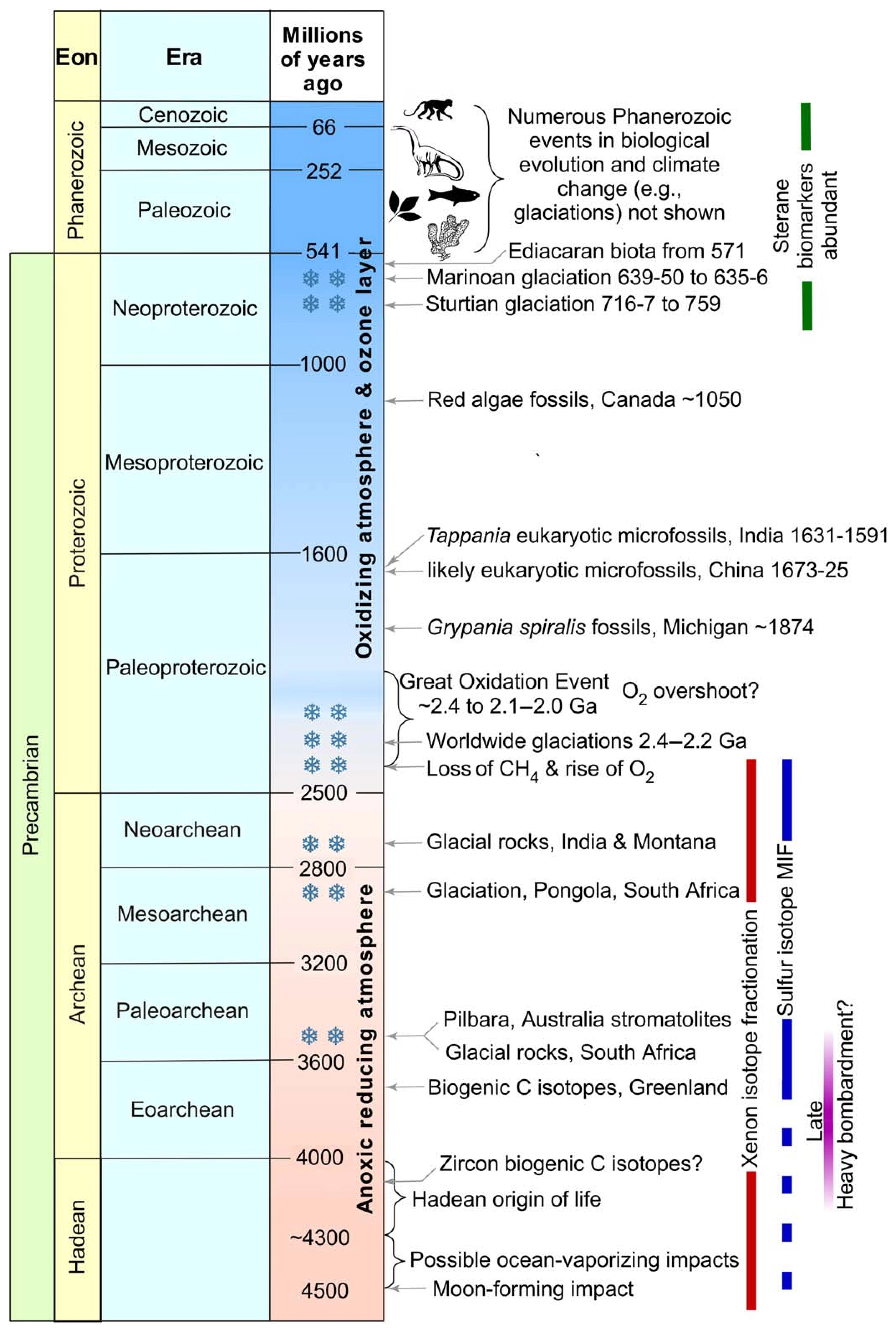
Fig. 9.11 Geologic time scale of the Precambrian with the major environmental and biological events, from the Moon-forming impact and the earliest evidence for life through the Great Oxidation Event (\(\sim\)2.4 Ga) to the Neoproterozoic glaciations and the first Ediacaran biota. The left columns give the eons and eras; the annotations mark the atmospheric transition from an anoxic, reducing composition to an oxidising one with an ozone layer. Reproduced from Catling and Zahnle [2020].#
Carbonate platforms, formed primarily by the calcification of marine organisms over the past \(\sim\)540 Myr, represent a substantial planetary \(\mathrm{CO_2}\) sink. On Earth, total carbon stored in surface and crustal reservoirs is on the order of \(10^{20}\) kg, equivalent to a \(\mathrm{CO_2}\) partial pressure of \(\sim 100\) bar if returned to the atmosphere [Catling and Kasting, 2017]. This is comparable in order of magnitude to the \(92\) bar of \(\mathrm{CO_2}\) in the present-day Venus atmosphere. Earth and Venus probably acquired comparable carbon inventories during accretion. Earth stored its carbon in carbonates, but Venus retained it in the atmosphere. The link between the biosphere and biosignatures (spectroscopic signatures of life used to characterise exoplanets) is taken up in Lecture 13 and Lecture 14.
9.1.10. The history of life on Earth#
The oldest accepted fossils are stromatolites at \(3.48\) Ga [Catling and Zahnle, 2020], while the origin of life and Precambrian biosignatures are evaluated in Lecture 14. Modern stromatolites in Shark Bay (Fig. 9.12) provide an analogue for this dominant early life form. Life arose within a billion years after liquid oceans formed at \(4.3\) to \(4.4\) Ga. Yet microbes dominated alone for \(3\) Gyr. Complex life, punctuated by mass extinctions like the end-Cretaceous impact at \(66\) Ma (Lecture 12), spans only the final \(12\%\) of Earth’s history (Fig. 9.13).
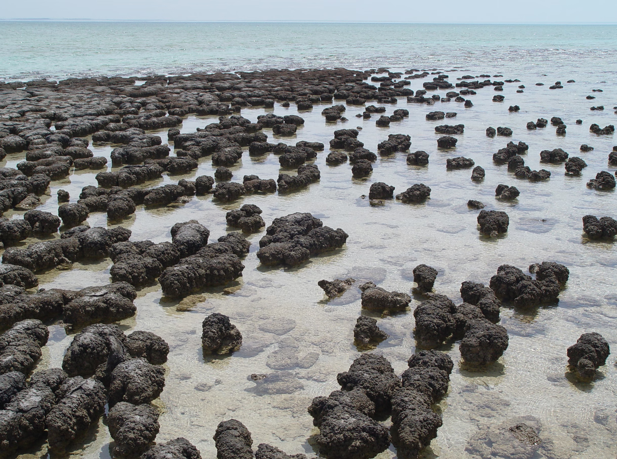
Fig. 9.12 Modern stromatolites in the hypersaline waters of Shark Bay, Western Australia. Microbial mats trap and bind sediment into these layered mounds; fossil stromatolites of the same construction, dated to \(3.48\) Ga in the nearby Pilbara region, are the oldest widely accepted evidence for life on Earth. Photo by Paul Harrison (Wikimedia Commons), CC BY-SA 3.0.#
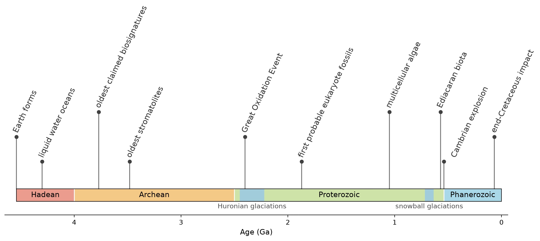
Fig. 9.13 Major events in the history of life on Earth, plotted on the geologic eon strip. Stemmed markers give representative ages for the milestones discussed in the text, from the formation of Earth and the first liquid water oceans through the earliest biosignatures, the Great Oxidation Event, the first eukaryotes and multicellular algae, to the Ediacaran biota, the Cambrian explosion, and the end-Cretaceous impact. Blue bands on the strip mark the Huronian and Neoproterozoic snowball glaciations. Event ages are representative values from the cited literature [Catling and Zahnle, 2020, Dodd et al., 2017, Gibson et al., 2018, Hoffman et al., 2017, Javaux and Lepot, 2018, Lyons et al., 2014, Mojzsis et al., 1996, Nutman et al., 2016]; eon boundaries follow Gradstein et al. [2020]. Course-original figure.#
This history offers two lessons for planetary science. First, because life arose fast while complexity arose slowly, microbial biospheres may be far more common than complex ones (Lecture 13, Lecture 14). Second, atmospheric oxygen was negligible during life’s first \(2\) Gyr. The inhabited Archean Earth therefore lacked an oxygen biosignature. Both points build on the record in Fig. 9.10.
9.2. Part 2: Venus, the alien twin#
9.2.1. Venus overview: why it is the twin and why it is not#
Venus is the second planet from the Sun, with a semimajor axis of \(0.723\) AU, mass \(0.815\, \Mearth\), radius \(0.950\, \Rearth\), and mean density \(5.24\) g/cm\(^3\) [NASA Jet Propulsion Laboratory, 2026]. By bulk measure, Venus is Earth’s near-twin with a silicate mantle and iron core.
However, its surface and atmospheric conditions contrast sharply with Earth (Fig. 9.14). Surface pressure is \(92\) bar and surface temperature reaches \(737\) K. The atmosphere is \(96.5\%\) \(\mathrm{CO_2}\) and \(3.5\%\) \(\mathrm{N_2}\), with sulfuric acid (\(\mathrm{H_2SO_4}\)) cloud droplets between \(48\) and \(70\) km altitude. Venus exhibits retrograde rotation (rotation against the orbital direction). The sidereal period is \(243.0\) Earth days and the solar day \(116.75\) Earth days. It lacks a global magnetic field. The internal dipole upper limit is \(10^{-5}\) of Earth’s field [Smrekar et al., 2018]. The water inventory is only \(20\) to \(30\) ppm (\(1\) to \(3\) cm equivalent depth). That is roughly \(10^5\) times less than Earth’s \(2.7\) km.
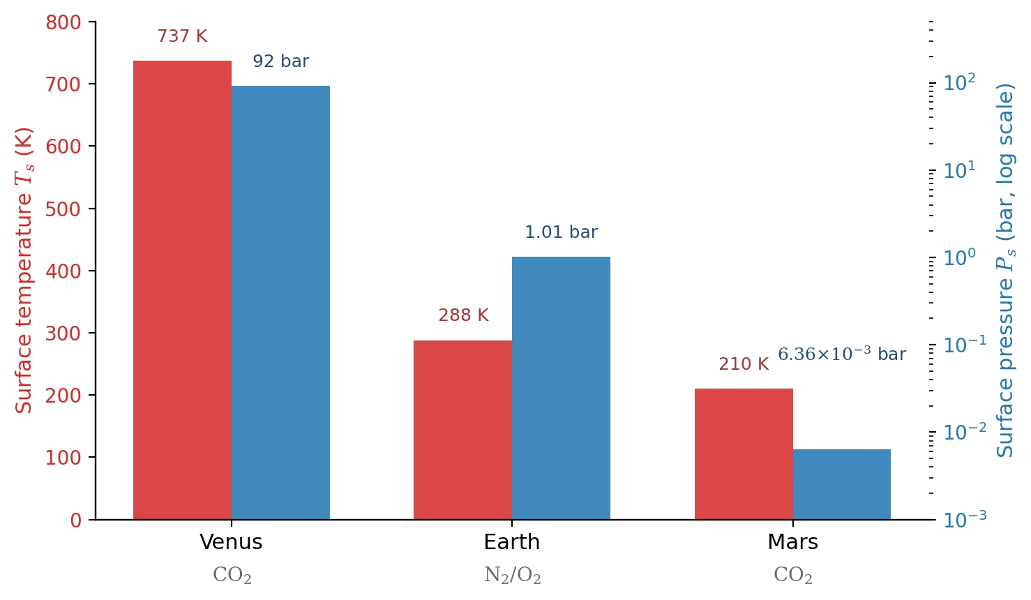
Fig. 9.14 Surface temperature (red bars, left axis) and surface pressure (blue bars, right axis, logarithmic) of Venus, Earth and Mars, with the dominant gas below each. Venus and Earth, near-twins in bulk, differ by a factor of 92 in surface pressure and by about 450 K at the surface; Mars is shown for comparison. Data from [NASA Jet Propulsion Laboratory, 2026]. Course-original figure.#
9.2.2. Exploring Venus: the mission history#
Venus exploration relies on three primary data sources: in-situ entry probes, orbital radar mapping, and orbital spectroscopy. In-situ measurements by Soviet Venera landers and Pioneer Venus probes established the \(92\) bar, \(737\) K surface state, basaltic chemistry, and noble-gas abundances (Fig. 9.15).
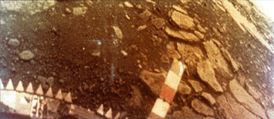
Fig. 9.15 The surface of Venus photographed by the Soviet Venera 13 lander on 1 March 1982 under the 92-bar, 737 K atmosphere, showing flat basaltic rock slabs and dark soil. Venera 13 survived for 127 minutes in the supercritical \(\mathrm{CO_2}\) environment, returning colour panoramic views of the Venusian surface. Credit: USSR / NASA NSSDC, public domain.#
Magellan mapped \(\sim\)98% of the surface at \(\sim\)100 m resolution using synthetic-aperture radar (radar imaging that penetrates cloud cover). This mapping provides the global topographic dataset for Venus geology. ESA’s Venus Express (\(2006\)–\(2014\)) measured atmospheric dynamics, surface thermal emission, and hydrogen and oxygen escape rates; JAXA’s Akatsuki (\(2015\) to present) images the cloud dynamics in the ultraviolet and infrared. Because no orbital mission flew between 1994 and 2006 and no in-situ probe has visited since 1985, the planetary dataset has substantial observational gaps. Three new orbiters and probes planned for the 2030s (NASA’s VERITAS and DAVINCI, and ESA’s EnVision) aim to resolve these questions.
9.2.3. Venus surface morphology#
The primary diagnostic observation of Venus’ surface is its hypsometry, the statistical distribution of surface elevations across a planet. Earth displays a bimodal hypsometry because plate tectonics produces low basaltic ocean basins (around \(-4\) km) and high granitic continents (around \(0\) to \(+1\) km) in distinct isostatic equilibria. In contrast, Venus exhibits a unimodal hypsometry with a single broad elevation peak and no continent-ocean dichotomy. This unimodal distribution indicates that Venus lacks Earth-like plate tectonics [Smrekar et al., 2018].
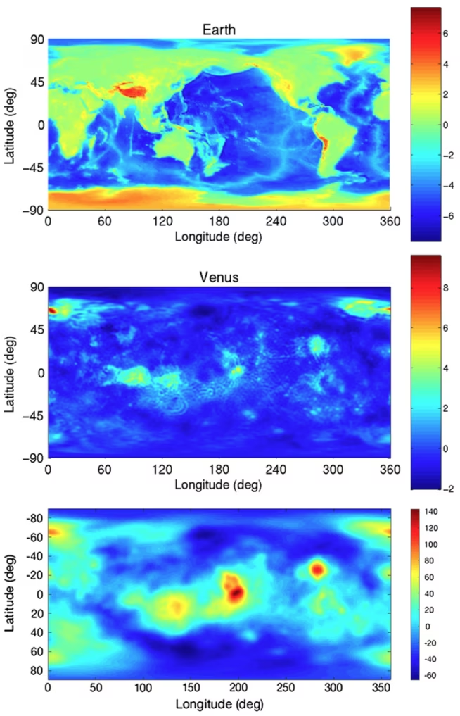
Fig. 9.16 Topography of Earth (top) and Venus (middle) and geoid of Venus (bottom). The top two colour bars give surface elevation in km, relative to sea level for Earth and to the mean planetary radius for Venus; Earth is shown at the same spatial resolution as the Magellan data for Venus. The bottom colour bar gives the geoid height in m, computed from the Magellan gravity field. In the bottom panel north is up, as in the panels above, but the latitude labels have the wrong sign: Beta Regio (about \(25^\circ\)N, \(283^\circ\)E) is the geoid high labelled near \(-25^\circ\). Venus’ unimodal hypsometry contrasts with Earth’s bimodal distribution; reproduced from Smrekar et al. [2018].#
The surface of Venus is dominated by volcanic plains, broad flood-basalt expanses that cover about \(80\%\) of the planet (Fig. 9.17). Embedded within these plains are tesserae, elevated plateaus covering roughly \(8\%\) of the surface that represent the oldest mapped terrain and record complex tectonic deformation; near-infrared emissivity suggests that some tesserae may be felsic, which would indicate ancient water-rock interaction [Widemann et al., 2023].
Coronae are circular volcano-tectonic structures unique to Venus (\(100\)–\(1000\) km in diameter) representing the surface expression of upwelling mantle plumes. These structures reflect stagnant-lid volcanism, where internal heat escapes through localized plumes rather than plate-tectonic recycling. Gravity observations indicate that some coronae overlie active mantle plumes today.
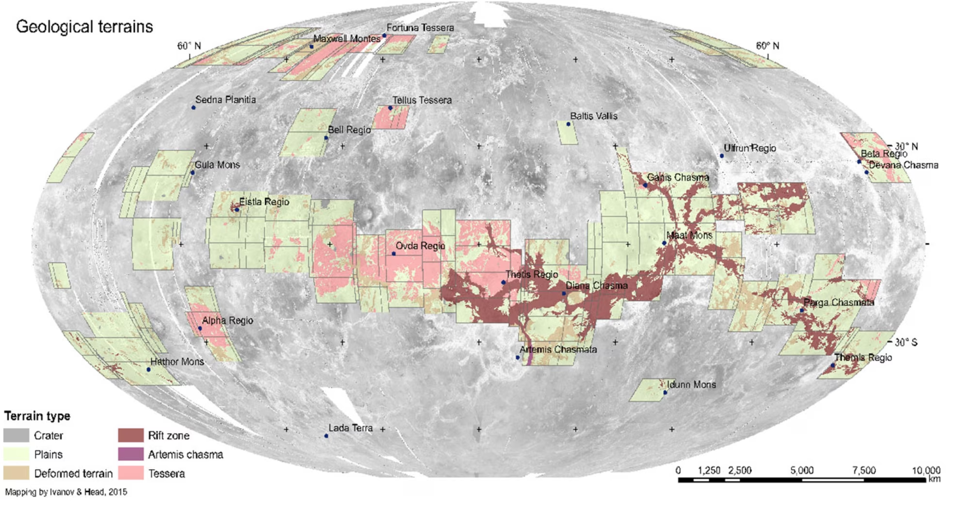
Fig. 9.17 Global geological-terrain map of Venus overlaid on a Magellan radar mosaic. Terrain classification after Ivanov and Head [2015]; reproduced from Widemann et al. [2023].#
A low impact crater density across Venus corresponds to a young average crater retention age of \(150\)–\(250\) Myr, implying that widespread resurfacing erased earlier craters [Smrekar et al., 2018]. Resurfacing models range from catastrophic global overturn \(\sim\)500 Myr ago to steady-state volcanic renewal, with intermediate episodic regional resurfacing favoured by random crater distributions [Widemann et al., 2023].
9.2.4. Venus interior and tectonic regime#
Venus’ interior structure is inferred primarily from gravity data, rotation rate, and theoretical extrapolation from Earth. The Magellan gravity field (Fig. 9.16), mapped to spherical harmonic degree \(\sim\)70, correlates strongly with long-wavelength topography, indicating dynamic support by deep mantle plumes and downwellings [Smrekar et al., 2018].
Given its similar uncompressed bulk density, Venus likely has an Earth-like bulk composition with an iron-nickel core, silicate mantle, and basaltic crust. However, because slow rotation makes the moment of inertia difficult to determine, core state remains unknown, and we lack evidence for inner-core nucleation (solid-core crystallisation from liquid metal).
Present-day Venus operates in a stagnant-lid regime, where the lithosphere forms a single globally connected shell without plate boundaries or subduction zones. As discussed in Lecture 7, tectonic regimes depend strongly on water content because mantle dehydration stiffens rock. Mantle dehydration following water loss likely raised viscosity, locking Venus into a stagnant lid as it dried (Fig. 9.18).
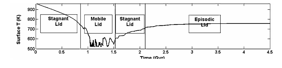
Fig. 9.18 Surface temperature evolution of Venus over \(\sim\)4.5 Gyr from a numerical tectonic-regime model, from the bottom panel of Smrekar et al. [2018]. The boxed labels mark successive stagnant-lid, mobile-lid, stagnant-lid, and episodic-lid intervals. The episodic-lid phase produces the resurfacing pulses inferred from present-day crater statistics; the mantle-temperature and volcanic-production-rate panels of the same model (not reproduced here) show the corresponding pulses in interior heat transport.#
Alternatively, an episodic-lid model proposes that a normally stagnant lithosphere becomes unstable every \(\sim\)500 Myr, undergoing brief episodes of global subduction and volcanism before returning to stagnant behaviour. This model naturally explains the resurfacing inferred from crater statistics.
The absence of a Venusian magnetic field is also tied to its interior state (Lecture 4). For a planetary dynamo to operate, core convection requires either efficient thermal cooling by the mantle or compositional buoyancy from inner-core freezing. On Venus, the stagnant lid insulates the core and impedes heat flow across the core-mantle boundary, suppressing thermal convection. Without inner-core nucleation, the core would also lack compositional buoyancy, so inefficient core cooling under the stagnant lid and a possible lack of inner-core nucleation are the leading explanations for the absent dynamo.
9.2.5. Venus atmosphere: structure and dynamics#
The vertical structure of the Venusian atmosphere provides key contrasts with Earth that motivate the runaway greenhouse derivation following Lecture 5 and Lecture 6.
The composition is overwhelmingly \(\mathrm{CO_2}\) (\(96.5\%\)), with \(\mathrm{N_2}\) (\(3.5\%\)) the only other major species. Trace gases include \(\mathrm{SO_2}\) at \(\sim\)150 ppm, water vapour at \(\sim\)30 ppm, and noble gases that preserve the history of volatile delivery and degassing. A high primordial \(^{36}\)Ar abundance shows that Venus holds a larger primordial noble-gas inventory than Earth [Lammer et al., 2018]. In contrast, the atmospheric \(^{40}\)Ar/\(^{36}\)Ar ratio of \(\approx 1.1\) (compared with \(\approx 300\) on Earth) indicates that only \(\sim 10\) to \(34\)% of radiogenic \(^{40}\)Ar has outgassed compared with \(\sim 50\)% on Earth, so Venus has outgassed less of its mantle volatile inventory [Gillmann et al., 2022].
The thermal profile is roughly adiabatic from the surface (\(T_s = 737\) K, \(P_s = 92\) bar) up to about \(65\) km altitude at the cloud tops. The atmospheric scale height, the characteristic vertical distance over which pressure decreases by a factor of \(e\), is about \(16\) km at the surface compared with \(\sim 8\) km on Earth. This difference is evaluated using the hydrostatic scale height from Lecture 5:
Plugging in \(T = 737\) K, \(m = 7.30 \times 10^{-26}\) kg for \(\mathrm{CO_2}\), and \(g = 8.87\) m/s\(^2\) gives \(H \approx 1.57 \times 10^4\) m, or \(\sim 16\) km (with the mean molecular weight \(43.4\) of the real atmosphere, \(15.9\) km). For Earth (\(T = 288\) K, \(m = 4.81 \times 10^{-26}\) kg, \(g = 9.81\) m/s\(^2\)), \(H \approx 8.4\) km. This factor-of-two difference is set primarily by the higher temperature ratio \(T_{\mathrm{Venus}} / T_{\mathrm{Earth}} \approx 2.55\), which outweighs the heavier molecular weight of \(\mathrm{CO_2}\). Above the clouds, temperature decreases through the mesosphere and rises in the thermosphere where solar EUV is absorbed (Fig. 9.19).
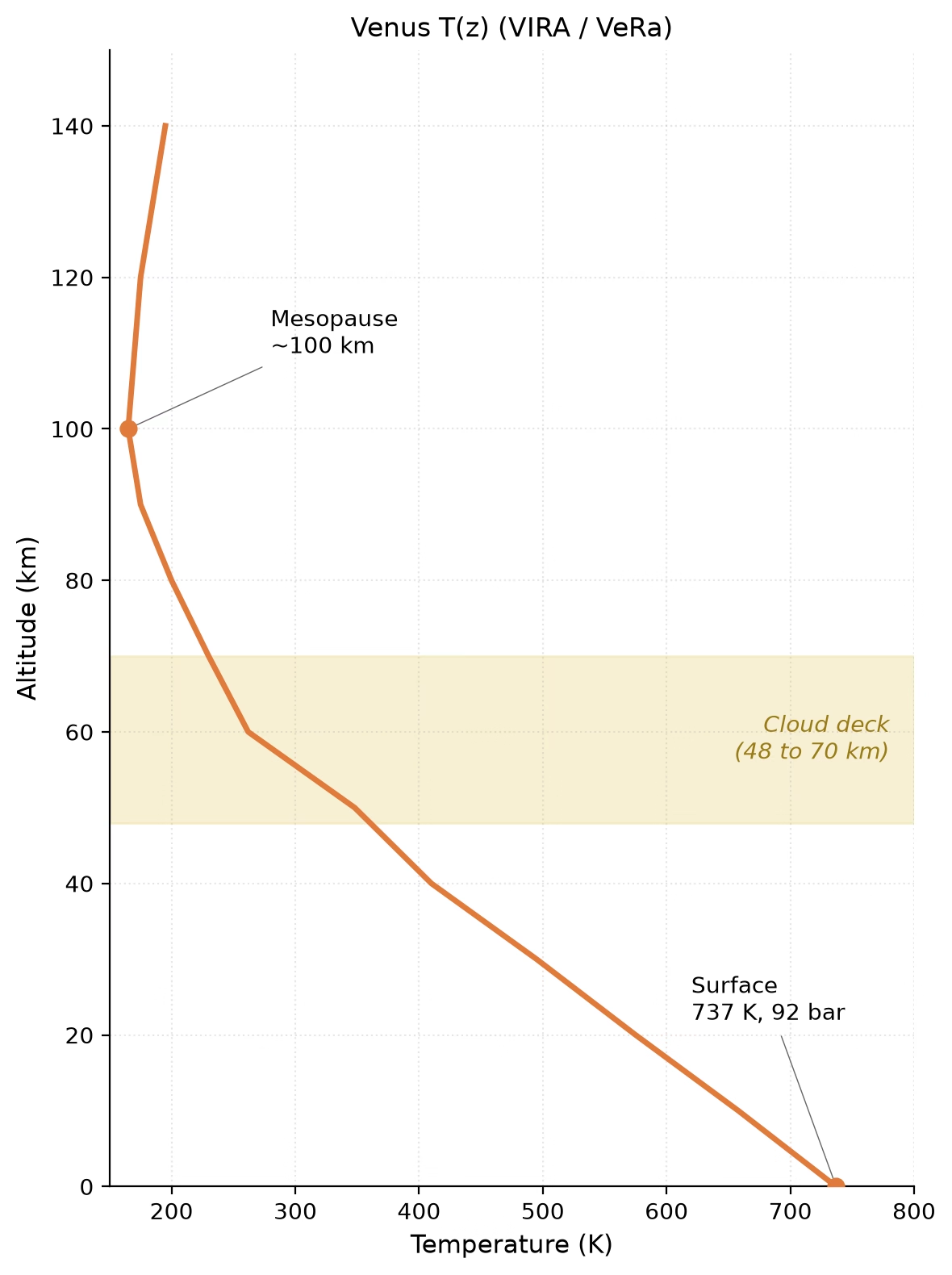
Fig. 9.19 Venus temperature profile from the 737 K, 92 bar surface through the cloud deck (48 to 70 km, shaded) to the mesopause near 100 km, from Pioneer Venus / VIRA data [Seiff et al., 1985] below and Venus Express radio occultations [Tellmann et al., 2009] above; no ozone inversion interrupts the monotonic fall, and the deep troposphere is close to adiabatic. Pedagogical fit, course-original figure; Lecture 5 compares the same profile with Earth and Titan.#
The cloud system consists of three vertically stacked layers between roughly \(48\) and \(70\) km altitude. Solar UV photolyses \(\mathrm{SO_2}\) to form \(\mathrm{SO_3}\). This combines with water vapour to produce \(\mathrm{H_2SO_4}\) droplets. These clouds are optically thick with a visible-band albedo of \(\sim 0.77\). They form the effective radiating surface at visible and near-IR wavelengths. An unidentified UV absorber produces banded features at the cloud tops, while contested trace detections such as phosphine (\(\mathrm{PH_3}\)) were examined in Lecture 6.
Atmospheric circulation is dominated by super-rotation, where the atmosphere rotates substantially faster than the underlying solid planet. The cloud-top atmosphere circles Venus in roughly \(4\) Earth days (moving roughly \(60\) times faster than the surface), in a direction opposed to the solid planet rotation of \(243\) Earth days. Maintaining this circulation against surface friction requires upward angular momentum transport by thermal tides and planetary-scale waves.
9.2.6. The runaway greenhouse and how Venus locked into it#
A one-layer grey greenhouse model (Lecture 5) gives:
yielding \(T_s \approx 1.19\, T_{\mathrm{eq}}\). For Earth (\(S_\oplus = 1361\) W/m\(^2\), \(A = 0.30\)), this gives \(T_s \approx 303\) K, close to the observed \(288\) K. For Venus (\(S_{\mathrm{Venus}} = 2604\) W/m\(^2\), \(A \approx 0.77\)), \(T_{\mathrm{eq}} \approx 227\) K and the one-layer model predicts \(T_s \approx 270\) K; the observed surface temperature of \(737\) K exceeds \(T_{\mathrm{eq}}\) by \(\Delta T \approx 510\) K, against Earth’s \(33\) K. The observed Venus surface temperature of \(737\) K is far hotter than predicted. The reason is that a dense atmosphere lifts the infrared photosphere far above the surface.
Warming increases atmospheric water vapour via the Clausius-Clapeyron relation. This strengthens the greenhouse effect. When absorbed solar flux exceeds the maximum outgoing longwave radiation (OLR) that a moist atmosphere can emit, the planet enters a runaway greenhouse, a state where oceans evaporate completely. This upper bound is the Simpson-Nakajima limit, the maximum OLR a water-rich atmosphere can radiate to space (Nakajima et al. [1992]; Fig. 9.20, Fig. 9.21).
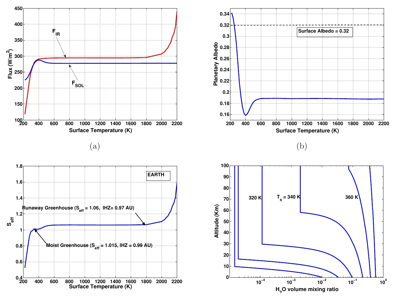
Fig. 9.20 Climate-model calculation of the runaway greenhouse limit and the inner edge of the habitable zone for an Earth-like planet (Kopparapu et al. [2013] Fig. 3), showing outgoing longwave radiation asymptoting to \(\sim 291\) W/m\(^2\) at high surface temperatures compared to the line-by-line value of \(\sim 282\) W/m\(^2\) from Goldblatt et al. [2013]. Radiative equilibrium yields the runaway greenhouse limit at \(S_{\mathrm{eff}} = 1.06\) (inner habitable-zone edge at \(\sim 0.97\) AU for present-day solar luminosity) and the moist greenhouse limit at \(S_{\mathrm{eff}} = 1.015\) (\(\sim 0.99\) AU), with water vapour mixing ratio profiles plotted for \(T_s = 320\), \(340\), and \(360\) K.#
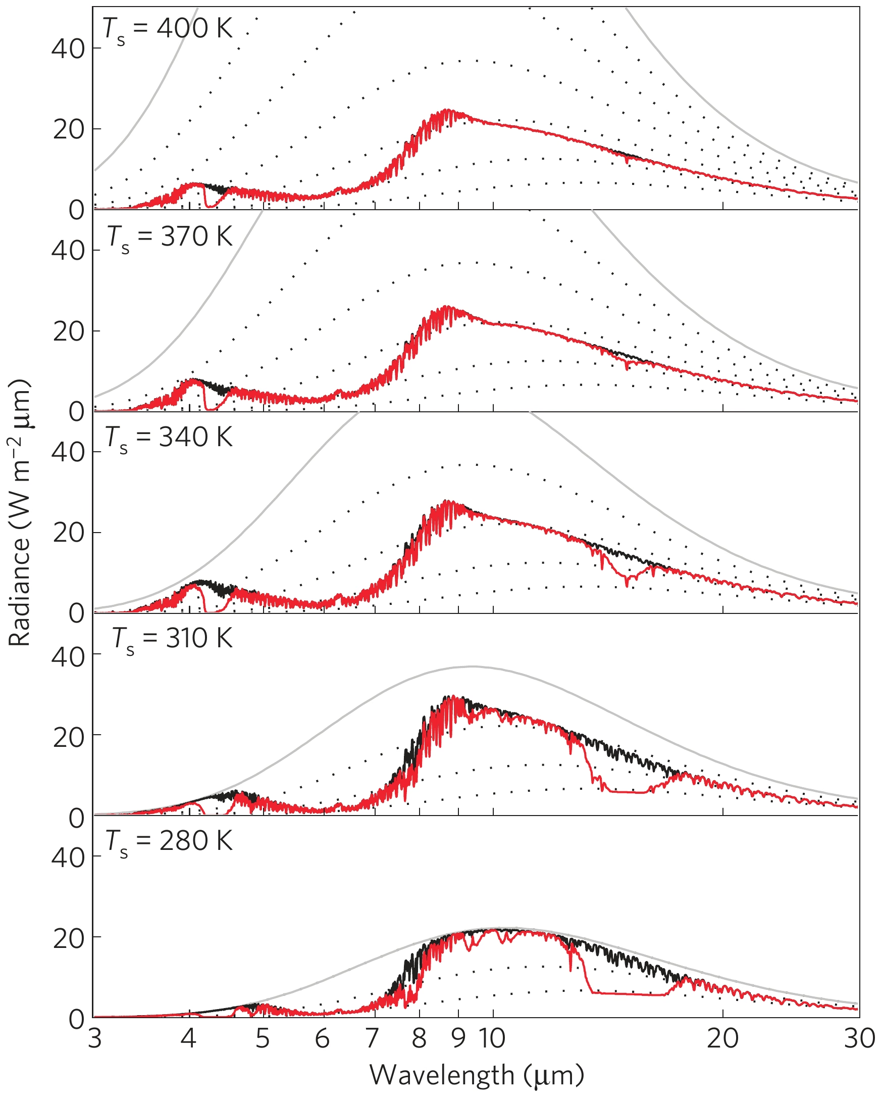
Fig. 9.21 Thermal-radiance spectra of an Earth-like atmosphere for surface temperatures \(T_\mathrm{s} = 280, 310, 340, 370, 400\) K (Goldblatt et al. [2013] Fig. 3(b)), comparing independent line-by-line calculations against blackbody curves as water vapour absorption closes the 8–14 \(\mu\)m atmospheric window. Above \(T_\mathrm{s} \sim 340\) K, the integrated outgoing flux saturates at the runaway-greenhouse asymptote of \(\sim 282\) W m\(^{-2}\), so that further surface warming cannot produce a compensating increase in thermal emission to space.#
Radiative transfer calculations place the Simpson-Nakajima limit at approximately \(280\text{--}310\) W/m\(^2\) [Goldblatt et al., 2013]. Earth absorbs about \(240\) W/m\(^2\), remaining below this limit. Venus, at \(0.723\) AU, receives \(1.91 \times\) more stellar flux per unit area, and with an Earth-like albedo it would absorb \(\sim 460\) W/m\(^2\). This exceeds the threshold. Upper-atmospheric water photolysed and hydrogen escaped to space. The result is the dry, \(\mathrm{CO_2}\)-dominated, \(737\) K surface observed today.
Fig. 9.22 shows the surface temperature of a steam atmosphere over a magma ocean as a function of the absorbed stellar and geothermal flux.
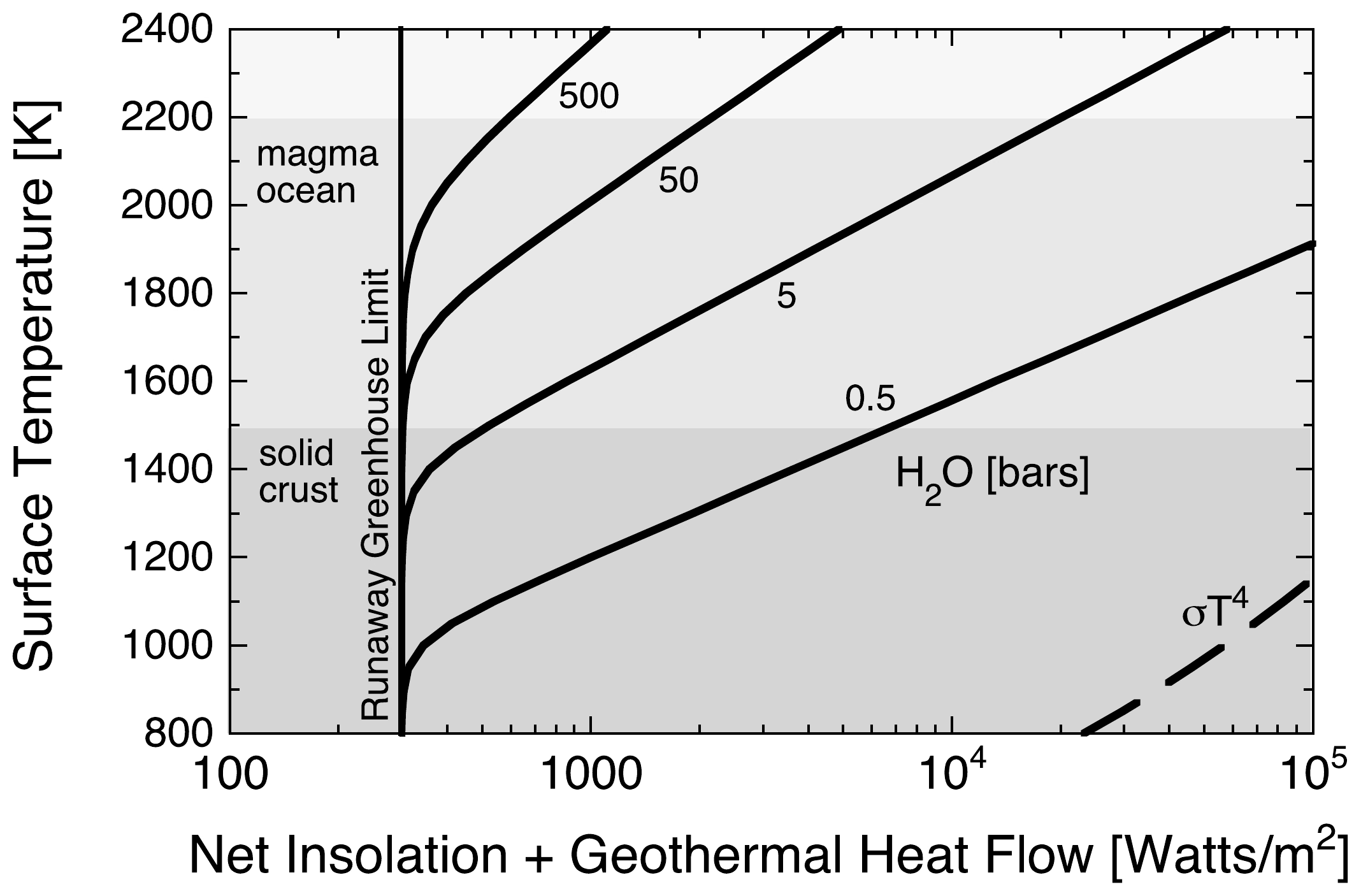
Fig. 9.22 Surface temperature as a function of net insolation plus geothermal heat flow for a steam atmosphere over a magma ocean, from Zahnle et al. [2007] (after Kasting [1988] and Abe & Matsui 1988). The radiated cooling rate is equal to the sum of absorbed sunlight and geothermal heat flow. The plot shows the surface temperature as a function of this combined heat input for different amounts of atmospheric \(\mathrm{H_2O}\) (in bars). The runaway greenhouse threshold appears as a vertical boundary near \(\sim\)300 W/m\(^2\) on the heat-flow axis (the “Runaway Greenhouse Limit” line in the figure): no steady state with a solid crust exists to its left, and for net heat fluxes only modestly above this value the surface stays molten beneath a thick steam atmosphere. Reproduced from Zahnle et al. [2007].#
9.3. Blackboard derivation: The Simpson-Nakajima runaway greenhouse limit#
Blackboard derivation: the Simpson-Nakajima limit
Goal: Show that the outgoing longwave radiation from a water-rich atmosphere has a maximum value, set by the saturation vapour pressure profile, that is independent of the surface temperature above some threshold.
Setup. Consider a water-rich planet with a wet adiabatic atmosphere. The water vapour partial pressure is everywhere set by the local saturation vapour pressure \(p_{\mathrm{sat}}(T)\), given by the Clausius-Clapeyron relation:
where \(L \approx 2.5 \times 10^6\) J/kg is the latent heat of vaporisation of water and \(R_v = 461\) J/(kg K) is the specific gas constant for water vapour. Integrating gives the familiar exponential dependence:
with \(p_{\mathrm{ref}} = 611\) Pa and \(T_{\mathrm{ref}} = 273.16\) K (the triple point of water, rounded to \(273\) K below). The column is pure water vapour and saturated at every level, the surface included, so the surface pressure is the saturation pressure at the surface temperature: \(p_s = p_{\mathrm{sat}}(T_s)\); a hotter ocean puts exponentially more vapour into the column.
Fig. 9.23 shows the column that Steps 1 to 3 below work through: the surface at \(T_s\), the level where the infrared optical depth reaches \(\tau \sim 1\), and the outgoing flux \(\sigma T_{\mathrm{phot}}^4\) from that level.
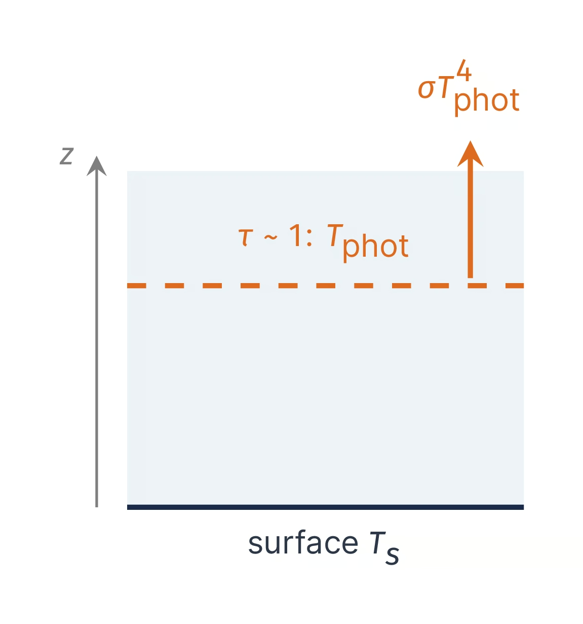
Fig. 9.23 Setup sketch of the board derivation of the Simpson-Nakajima limit: a saturated water-vapour column above a surface at temperature \(T_s\), the photosphere level where the infrared optical depth from the top reaches \(\tau \sim 1\) at temperature \(T_{\mathrm{phot}}\), and the outgoing longwave flux \(\sigma T_{\mathrm{phot}}^4\) that leaves from there. Course-original figure.#
Step 1: The IR optical depth and the photosphere temperature. The outgoing longwave radiation emerges from a thermal photosphere, defined as the level where the IR optical depth, integrated downward from the top of the atmosphere, reaches order unity. For a vertically uniform absorption coefficient \(\kappa\) (the effective infrared mass absorption coefficient of water vapour, with units of m\(^2\)/kg), the photosphere lies at column density \(N_{\mathrm{phot}} \sim 1/\kappa\).
Because water vapour is a strong IR absorber over a wide range of wavelengths, the photosphere of a water-rich atmosphere is set by the water vapour column density alone. At the photosphere, the water vapour pressure is set by Clausius-Clapeyron at the local temperature \(T_{\mathrm{phot}}\):
where \(g\) is the surface gravity. This equation says: the photosphere occurs at the level where the saturation vapour pressure equals the local hydrostatic pressure required to give an optical depth of order unity.
To solve Eq. (9.3) for \(T_{\mathrm{phot}}\), substitute the Clausius-Clapeyron form of the saturation curve and take the logarithm of both sides:
Collecting the \(1/T_{\mathrm{phot}}\) term on one side, \(\frac{L}{R_v T_{\mathrm{phot}}} = \ln(p_{\mathrm{ref}} \kappa / g) + L/(R_v T_{\mathrm{ref}})\), and inverting:
For Earth-like values (\(g = 10\) m/s\(^2\), and a band-averaged \(\kappa \sim 5 \times 10^{-2}\) m\(^2\)/kg representative of the strong rotational and vibrational water-vapour bands), this gives \(T_{\mathrm{phot}} \approx 258\) K.
Step 2: The outgoing longwave radiation. The OLR is approximately the blackbody emission at \(T_{\mathrm{phot}}\):
where \(\sigma = 5.67 \times 10^{-8}\) W/(m\(^2\) K\(^4\)) is the Stefan-Boltzmann constant.
The crucial observation is that \(T_{\mathrm{phot}}\) depends on the atmospheric properties (the absorption coefficient \(\kappa\) and the gravity \(g\)) and on the water vapour saturation curve, but not on the surface temperature. As the surface warms, the photosphere just moves to a higher altitude (because the saturation curve is exponentially steep), and its temperature stays clamped near the value set by Eq. (9.4). Fig. 9.24 shows this for four surface temperatures.
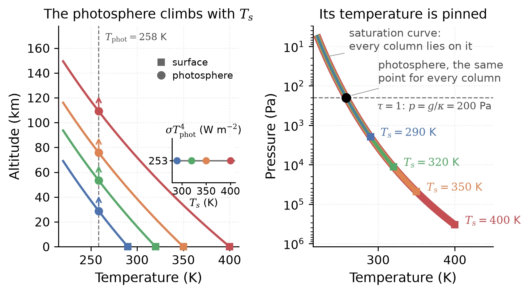
Fig. 9.24 The infrared photosphere of a saturated steam atmosphere for surface temperatures of \(290\), \(320\), \(350\) and \(400\) K, in the grey model of this derivation (\(\kappa = 0.05\) m\(^2\)/kg, \(g = 10\) m/s\(^2\), \(T_{\mathrm{ref}} = 273\) K). Left: temperature against altitude. A saturated pure-steam column in hydrostatic balance follows \(z = (L/g)\ln(T_s/T)\), a lapse rate of only \(gT/L \approx 1.0\) to \(1.6\) K/km between the photosphere and the surface, because latent heat dominates the energy budget of the column. The photosphere (circles), where \(p = g/\kappa = 200\) Pa, rises from \(29\) to \(109\) km, but its temperature stays at \(T_{\mathrm{phot}} = 258\) K. The inset shows the consequence: the emitted flux \(\sigma T_{\mathrm{phot}}^4 = 253\) W/m\(^2\) is the same for every surface temperature. Right: pressure against temperature. Every column lies on the one Clausius-Clapeyron saturation curve, from its surface (squares) upward; the photosphere pressure is a horizontal line, and the two cross at one point. The constant latent heat overestimates the saturation pressure by about \(25\%\) at the boiling point, so the surface pressures are model values; a full radiative-transfer treatment raises the flux limit to \(280\) to \(310\) W/m\(^2\) (Step 3). Course-original figure.#
Step 3: The Simpson-Nakajima limit. Combining Eqs. (9.4) and (9.5) and plugging in numerical values:
A more careful radiative-transfer calculation, including the wavelength dependence of water vapour absorption and the wings of the rotational and vibrational bands, gives a refined value of \(280\text{--}310\) W/m\(^2\) [Goldblatt et al., 2013, Kasting, 1988, Kasting et al., 1993]. This is the Simpson-Nakajima limit: the maximum thermal flux that a water-saturated atmosphere can radiate to space.
Step 4: Habitable zone implications. Compare this to the absorbed stellar flux at Earth’s distance. With a present solar constant of \(S_\odot = 1361\) W/m\(^2\) and an Earth-like Bond albedo \(A = 0.30\):
Earth is comfortably below the runaway greenhouse limit, by about \(40\)–\(70\) W/m\(^2\). At the orbit of Venus, the same calculation gives \(F_{\mathrm{abs}}^{\mathrm{Venus}} \approx 460\) W/m\(^2\) (assuming an Earth-like albedo, which is wrong for present Venus but is the relevant comparison for an early ocean-bearing Venus), well above the limit. Setting \(F_{\mathrm{abs}} = F_{\mathrm{OLR}}^{\max}\) and solving for the orbital distance gives the runaway greenhouse limit, at \(0.84\)–\(0.97\) AU for present-day solar luminosity depending on radiative-transfer assumptions [Goldblatt et al., 2013, Kasting et al., 1993, Kopparapu et al., 2013]. The moist greenhouse limit, where enough water reaches the stratosphere for rapid hydrogen escape, lies slightly outside, at \(0.95\)–\(0.99\) AU [Kasting et al., 1993, Kopparapu et al., 2013]; together the two limits mark the inner edge of the classical habitable zone. Venus, at \(0.723\) AU, sits well inside the inner edge.
Key insight. The runaway greenhouse is not an artefact of one model or one parameter choice; it is a thermodynamic feature of the water phase diagram combined with the elementary physics of radiative transfer through a saturated atmosphere. The maximum OLR is set by the temperature where the water vapour saturation curve produces the right column density to give an IR optical depth of order unity, and that temperature, and hence the maximum flux, is essentially independent of the surface temperature. Once a planet’s absorbed stellar flux exceeds this limit, no steady state with liquid surface water is possible: the atmosphere cannot lose heat fast enough, the surface temperature rises, the ocean evaporates, and the runaway proceeds to completion. The boundary is one-way: there is no thermodynamic path back to the wet state without removing the water from the atmosphere, and the only natural removal mechanism is photodissociation followed by hydrogen escape, which is irreversible on geological timescales.
The numerical value of the Simpson-Nakajima limit, around \(280\) W/m\(^2\) from the line-by-line calculations of Goldblatt et al. [2013] and consistent with the Kopparapu et al.\ 2013 reanalysis, has implications well beyond Venus. It defines the inner edge of the classical habitable zone for any star at any age. For the present-day Sun, this corresponds to the runaway greenhouse limit at \(S_{\mathrm{eff}} = 1.06\) (about \(0.97\) AU), with the moist greenhouse limit slightly inside Earth’s orbit at \(S_{\mathrm{eff}} = 1.015\) (about \(0.99\) AU) [Kopparapu et al., 2013]. For a younger and fainter Sun (say at \(4\) Ga, with \(L_\star \approx 0.75 L_{\star,\mathrm{today}}\)), the inner edge sat closer to the Sun, near \(\sim 0.83\) AU. The inner habitable zone edge has therefore been moving outward over Solar System history as the Sun brightens. The question of whether Venus was once inside the habitable zone (and if so, for how long) becomes a question of when the receding inner edge crossed the orbit of Venus from the inside.
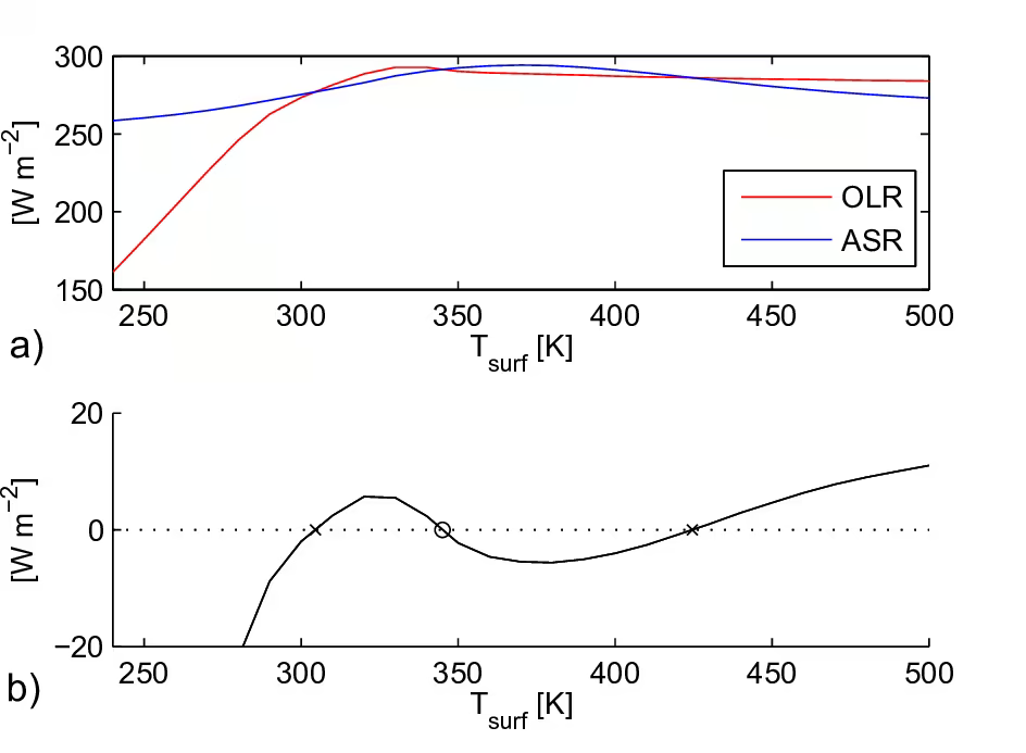
Fig. 9.25 OLR (red), ASR (absorbed shortwave radiation, blue), and OLR\(-\)ASR (bottom) as a function of surface temperature for an atmosphere with \(100\) ppm \(\mathrm{CO_2}\) at a stellar flux of \(F = 1.025\, F_0\), from Wordsworth and Pierrehumbert [2013]. There are three thermal equilibria (two stable, marked by crosses, and one unstable, marked by the open circle), illustrating that runaway-greenhouse atmospheres can have multiple solutions for the same incoming stellar flux. This bistability is one mechanism for the hysteresis between wet and dry climate states discussed below. Reproduced from Wordsworth and Pierrehumbert [2013].#
9.3.1. When did Venus lose its water?#
The Simpson-Nakajima limit makes a runaway greenhouse inevitable. The timing of the transition remains unresolved (Fig. 9.25).
In the early loss scenario, a primordial steam atmosphere prevents magma-ocean solidification, sustaining rapid water loss (Fig. 9.26) [Hamano et al., 2013] (Lecture 14).
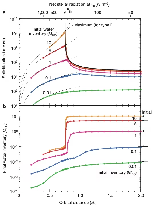
Fig. 9.26 The two types of terrestrial planet identified by Hamano et al. [2013] from coupled magma-ocean and atmosphere thermal-evolution models. Top panel: magma-ocean solidification time as a function of orbital distance (lower \(x\)-axis) and, equivalently, of net stellar radiation at the tropopause \(\tau_0\) (upper \(x\)-axis). Bottom panel: final water inventory retained on the planet. Coloured curves show different initial water inventories from 0.01 to 10 Earth-ocean masses (\(M_\mathrm{EO}\)). For orbital distances larger than the critical value \(a_\mathrm{cr} \approx 0.77\) AU (or net stellar radiation below the tropospheric limit \(F_\mathrm{lim}\)) the magma ocean crystallises within a few Myr and most of the initial water is retained: this is the Type I (Earth-like) regime. Inside \(a_\mathrm{cr}\) the solidification time diverges and the atmosphere loses essentially all its water to hydrodynamic escape: this is the Type II (Venus-like) regime. The sharp transition at \(a_\mathrm{cr}\) corresponds to the Simpson-Nakajima runaway-greenhouse threshold and provides a natural explanation for the Earth-Venus dichotomy. Reproduced from Hamano et al. [2013].#
Fig. 9.27 shows the coupled evolution of potential and surface temperature for a crystallising magma ocean under its steam atmosphere on a Venus-mass planet.
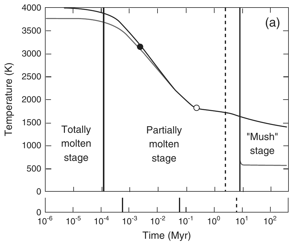
Fig. 9.27 Time evolution of potential temperature (black line) and surface temperature (grey line) for a crystallising magma ocean coupled to its outgassed steam atmosphere on a Venus-mass planet at the orbital distance of Venus, from panel (a) of Lebrun et al. [2013] Fig. 12. The three vertical regions (“totally molten”, “partially molten”, “mush”) track the planetary mantle as it crystallises; condensation of water vapour occurs at the boundary between the partially molten and mush stages. The dashed vertical line marks the time at which the magma ocean reaches \(98\%\) solidification, \(\sim 10\) Myr at Venus’ orbital distance (compared with \(\sim 1.5\) Myr at Earth’s and \(\sim 0.1\) Myr at Mars’ for the corresponding panels (b) and (c) of the same figure, not shown). The longer magma-ocean lifetime at smaller heliocentric distances gives the steam atmosphere ample time to photolyse and lose hydrogen to space, providing the foundation of the early-loss scenario for Venus. Lebrun et al. [2013] further showed (their Fig. 11, not shown) that below a critical distance of about \(0.66\) AU around a Sun-like star, an Earth-mass planet’s magma ocean cannot freeze at all and the planet remains molten indefinitely; Venus at \(0.72\) AU sits just outside this limit.#
In the late loss scenario, Venus condensed a surface ocean and remained temperate for billions of years [Way et al., 2016], and substellar clouds reflected sunlight until water loss occurred within the last \(\sim\)1 Gyr (Fig. 9.28).
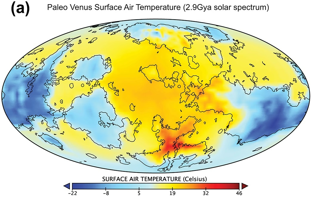
Fig. 9.28 Three-dimensional climate model simulation of the surface air temperature on a hypothetical paleo-Venus at \(2.9\) Ga with \(75\%\) of present solar irradiance, from panel (a) of Way et al. [2016] Fig. 2, plotted on a Mollweide global projection. Surface air temperatures range from \(-22^\circ\)C to a maximum of \(36^\circ\)C, with a global mean of \(11^\circ\)C, suggesting that an early Venus could have hosted long-lived liquid surface water. Way et al. [2016] confirmed similar temperate conditions for several variants (different epochs, modern Earth topography in place of Venusian topography, faster rotation), shown in panels (b)-(d) of the same figure (not reproduced here).#
Three-dimensional simulations show that water clouds preferentially form on the nightside (Fig. 9.29) [Turbet et al., 2021]. Nightside cloud warming prevents ocean condensation. This traps Venus in a runaway state (Fig. 9.30).
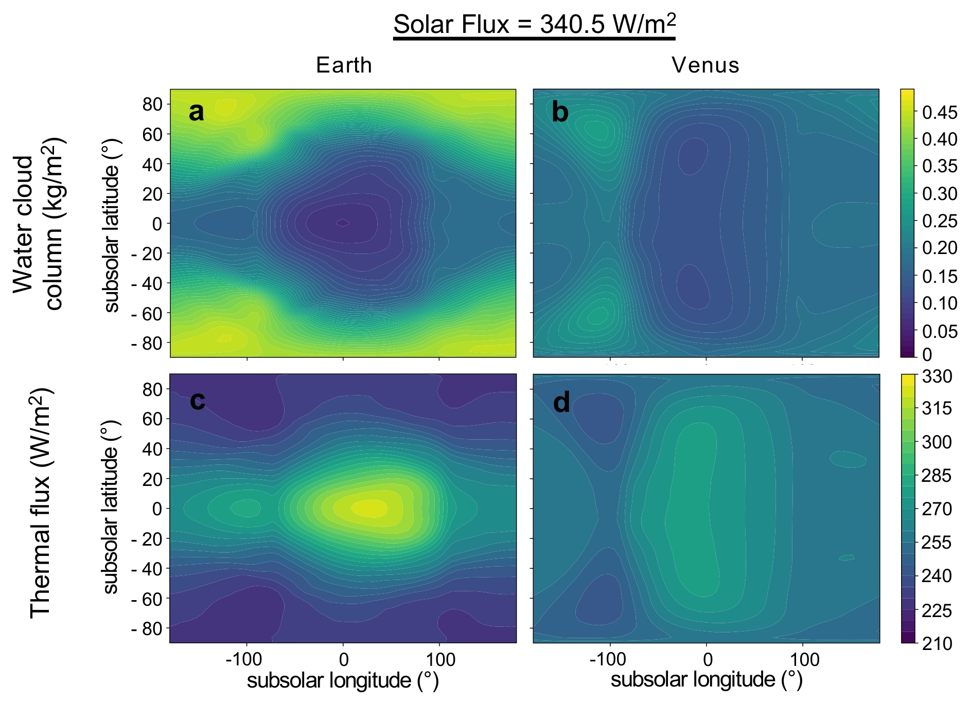
Fig. 9.29 Three-dimensional simulations of an initially hot and steamy Earth (a, c) and Venus (b, d), both forced to a stellar flux \(S = 340.5\) W/m\(^2\), the present-day Earth insolation. The upper row shows the vertically integrated water-cloud column and the lower row the thermal emission to space. The maps are in the heliocentric frame, so subsolar longitude \(0^\circ\) is the substellar point and \(\pm 180^\circ\) the antistellar point. In both cases the clouds are concentrated on the night-side, where they act as a greenhouse blanket and cut the thermal cooling to space, so the emission maps are anticorrelated with the cloud maps. The substellar region stays comparatively cloud-free, which keeps the planetary albedo low. The two planets rotate at very different rates, Earth with \(P_\mathrm{rot} \approx 24\) h and Venus with \(P_\mathrm{rot} \approx 5833\) h, about 243 times longer, yet the same night-side cloud pattern appears in both, so the mechanism does not depend on slow rotation. Reproduced from Turbet et al. [2021], Fig. 2a-d.#
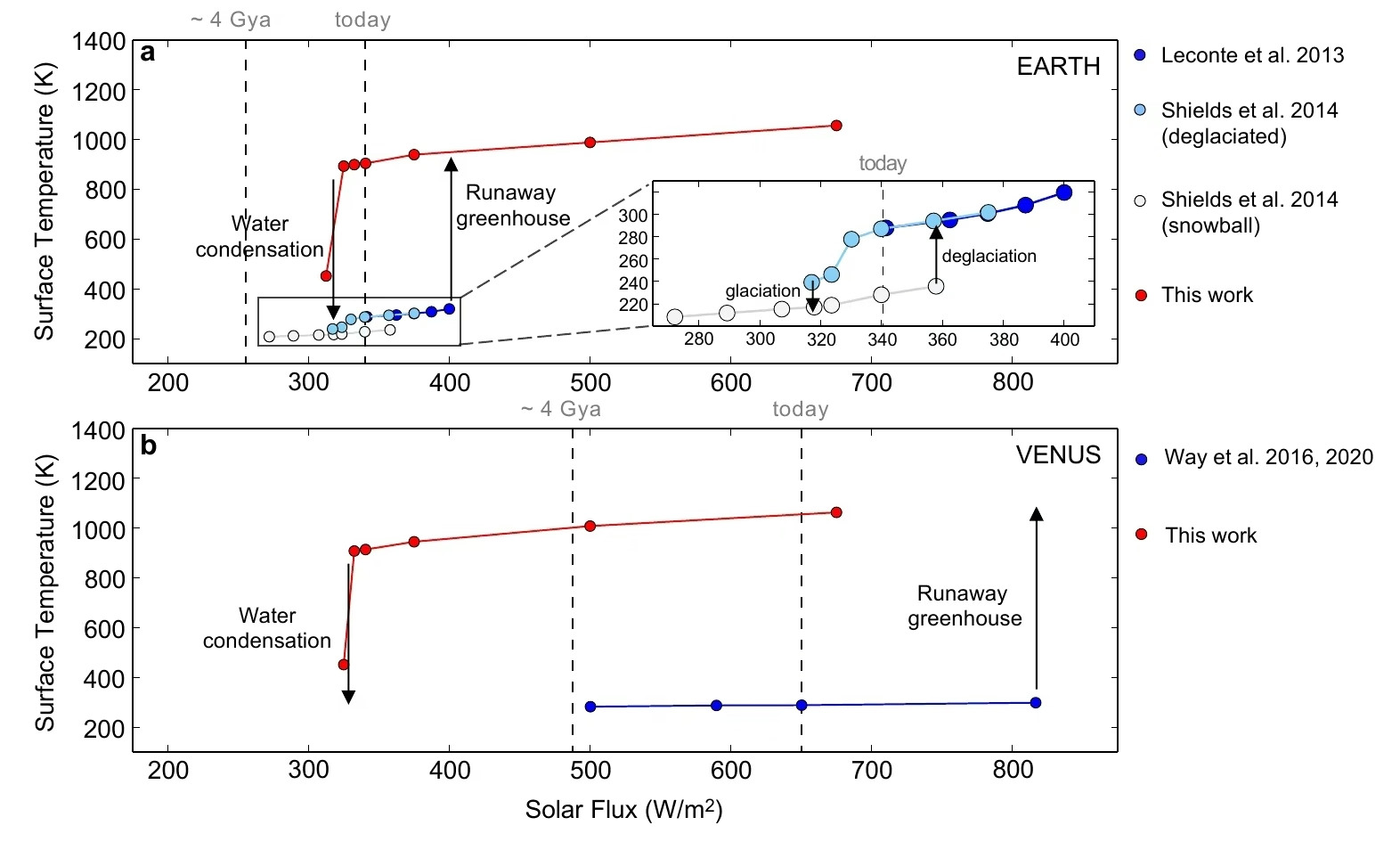
Fig. 9.30 Hysteresis loops for ocean formation on early Earth and Venus, from Turbet et al. [2021]. Panel (a) shows surface temperature as a function of incoming solar flux for Earth: at \(4\) Ga, water condenses from a steam atmosphere if the atmosphere is initially condensed (operating point near present-day) but enters the runaway greenhouse if it starts hot (red branch). Panel (b) shows the same for Venus: the runaway and condensed branches do not overlap, so an early Venus that started in the runaway state (the natural endpoint of magma ocean cooling at high solar flux) cannot reach the condensed branch even at \(4\) Ga, when the insolation at Venus was \(\sim\)25% lower than today and Venus still received \(\sim\)500 W/m\(^2\), well above the cloud-modified condensation threshold of \(\sim\)325 W/m\(^2\). Reproduced from Turbet et al. [2021], Fig. 4.#
Both early-loss and late-loss scenarios remain observationally untested (Fig. 9.31), and future measurements of noble gases and crustal composition may distinguish between an early ocean (Fig. 9.38) and a dry history (Fig. 9.32).
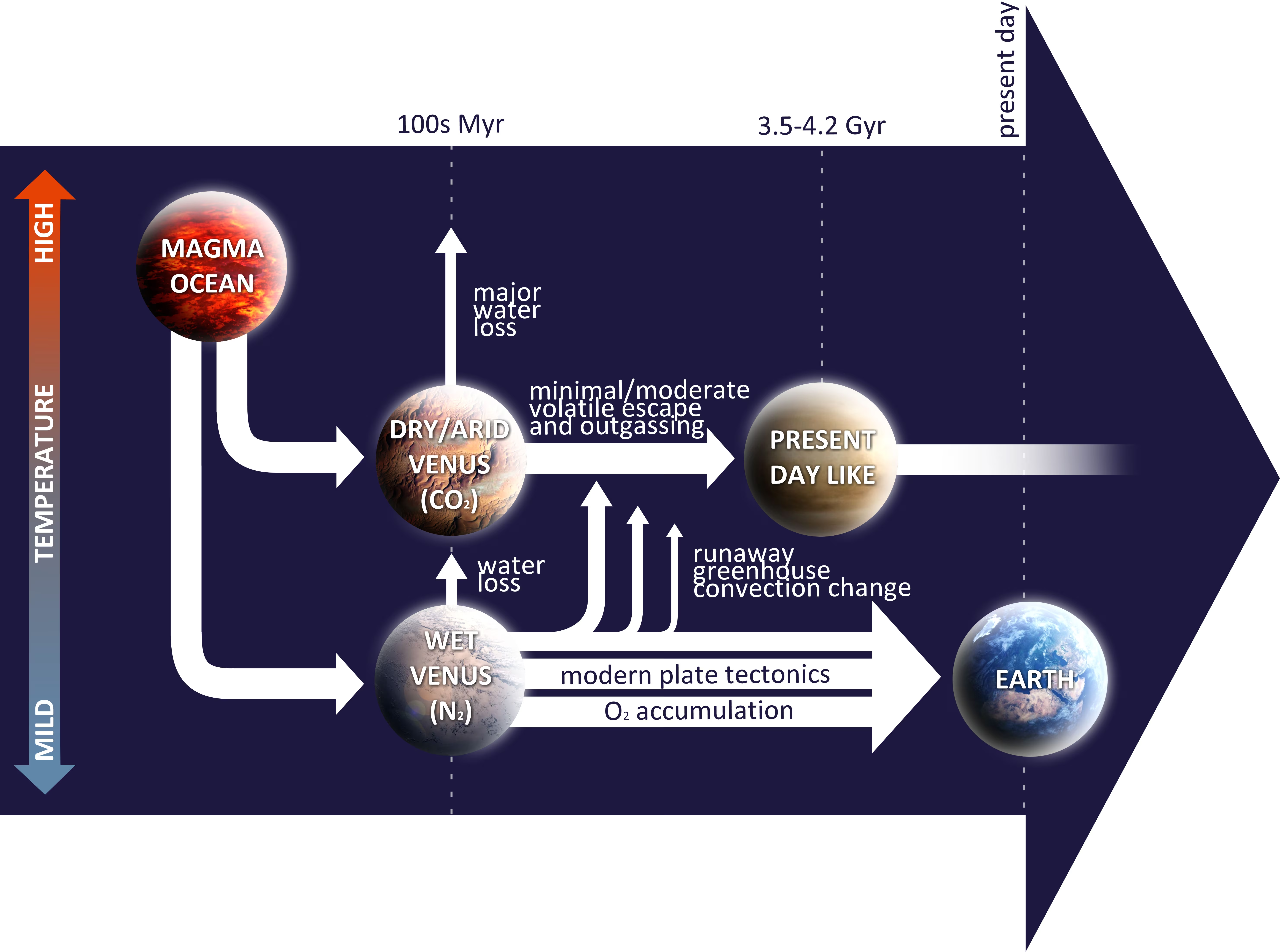
Fig. 9.31 The two main scenarios for Venus’ early evolution as summarised by Gillmann et al. [2022]. Top branch (Dry Venus, Hamano-style): the magma ocean never crystallises with a condensed surface, water photolyses early, and the planet emerges desiccated within \(\sim\)100 Myr. Bottom branch (Wet Venus, Way-style): the magma ocean crystallises, an ocean condenses, the planet remains habitable for several Gyr, and the runaway greenhouse is triggered later by gradual loss of water and the slow rise of solar luminosity. Both end at the present state of Venus, and current data cannot distinguish them definitively. Reproduced from Gillmann et al. [2022].#
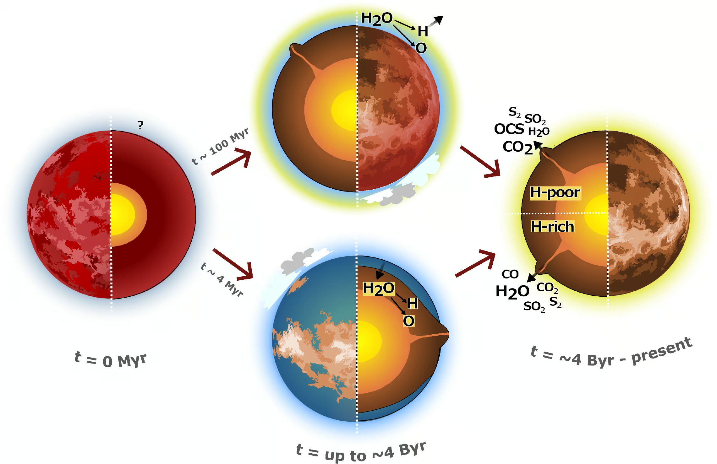
Fig. 9.32 The two dichotomous climate pathways for Venus from Constantinou et al. [2024], ending in interiors with very different water inventories. Upper branch (dry Venus): the planet emerges from its magma-ocean stage at \(t \approx 100\) Myr without ever condensing a surface ocean; water is lost early via photolysis and hydrogen escape, leaving an interior depleted in hydrogen and a present-day mantle that degasses S- and C-rich, \(\mathrm{H_2O}\)-poor volcanic gases. Lower branch (temperate, wet Venus): the magma ocean crystallises with a condensed ocean at the surface, the planet remains habitable for several Gyr, and the present-day mantle still contains significant water that emerges in \(\mathrm{H_2O}\)-rich volcanic gases. The two interior signatures map onto observable differences in the chemistry of Venus’ atmosphere. Constantinou et al. [2024] argue from the destruction rates of \(\mathrm{H_2O}\), \(\mathrm{CO_2}\), and \(\mathrm{OCS}\) in the present atmosphere that the volcanic source must be water-poor (at most \(\sim\)6% \(\mathrm{H_2O}\) mole fraction), favouring the dry-Venus branch. Reproduced from Constantinou et al. [2024].#
9.3.2. The D/H ratio: evidence for water loss#
The deuterium-to-hydrogen ratio (D/H) provides strong empirical evidence that Venus once possessed at least \(100\times\) more water than today. Early measurements gave an atmospheric \(D/H \approx 1.6 \times 10^{-2}\) for Venus, about \(100\) times the terrestrial standard mean ocean water value (\(D/H = 1.56 \times 10^{-4}\)) [Donahue et al., 1982], and later analyses revised the enrichment factor to \(\sim 150 \pm 30\) [Donahue et al., 1997].
Lighter hydrogen molecules acquire higher thermal velocities, so they escape more efficiently than deuterium. The remaining reservoir is progressively enriched in deuterium. This process follows Rayleigh distillation (isotopic fractionation during reservoir loss) [Hunten et al., 1987]. If \(f\) is the remaining hydrogen fraction and \(\alpha < 1\) is the fractionation factor (the ratio of deuterium to hydrogen escape efficiencies), the present isotopic ratio \(R\) relative to the initial ratio \(R_0\) obeys
The fractionation factor \(\alpha\) depends on the escape regime: \(\alpha \approx m_{\mathrm{H}}/m_{\mathrm{D}} \approx 0.5\) in the mass-ratio limit, and \(\alpha \approx \sqrt{m_{\mathrm{H}}/m_{\mathrm{D}}} \approx 0.71\) in the thermal-velocity limit. Setting \(R/R_0 = 150\) and solving \(f = 150^{1/(\alpha-1)}\) yields \(f_{\mathrm{mass}} \approx 150^{-2} \approx 4 \times 10^{-5}\) and \(f_{\mathrm{thermal}} \approx 150^{-3.4} \approx 4 \times 10^{-8}\). Multiplying the present water column (\(\sim 2\) cm of global equivalent layer) by \(1/f\) implies an initial inventory of several hundred metres for the mass-ratio case, but an unphysical several hundred kilometres (more than 100 Earth-ocean masses) for the thermal-velocity case. This contradiction shows that Venusian escape combined an early hydrodynamic phase with \(\alpha\) near unity and a later diffusion-limited phase that produced the observed enrichment. Under this lower-bound argument, the original Venusian water inventory was at least \(\sim 100\) times the present value.
The D/H ratio provides direct evidence that Venus lost most of its primordial water to space. Photolytic \(\mathrm{O_2}\) buildup and interior oxidation accompanied the loss (Fig. 9.33; Lecture 13, Lecture 14). However, D/H alone cannot determine whether water loss occurred early during a magma-ocean phase or over billions of years as solar EUV flux declined. Future noble gas measurements, particularly \(^{36}\)Ar/\(^{38}\)Ar and Xe isotopic ratios from the DAVINCI probe, will help distinguish between these escape histories.
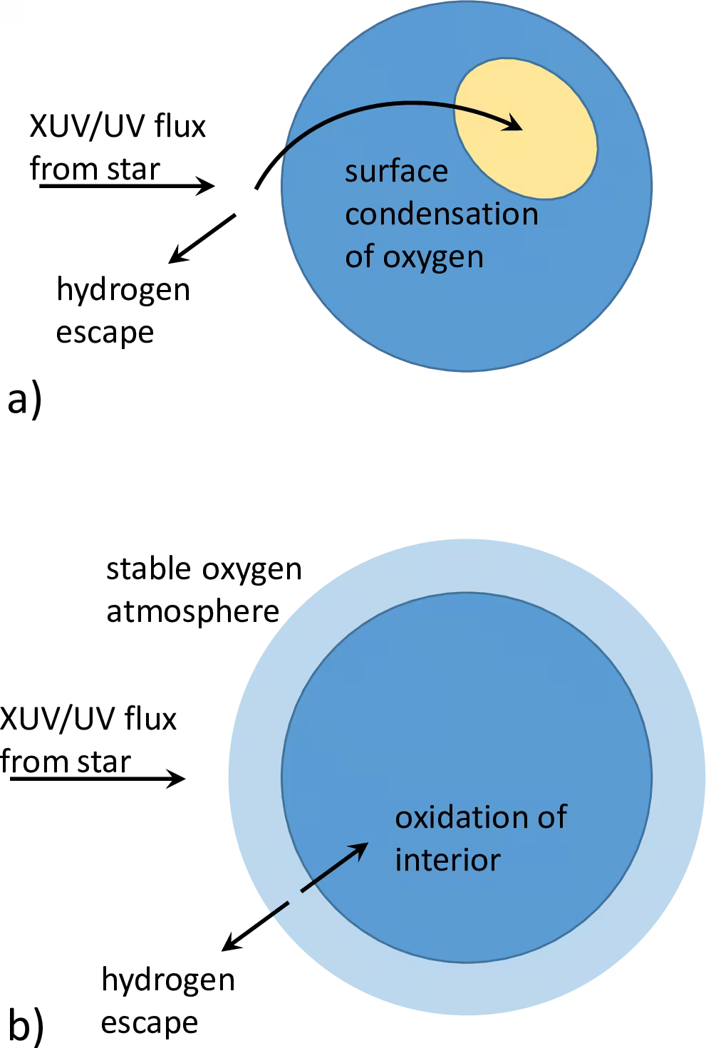
Fig. 9.33 Schematic of the abiotic build-up of an \(\mathrm{O_2}\)-dominated atmosphere by photolytic water loss on a terrestrial habitable-zone planet, from Wordsworth and Pierrehumbert [2014]. Top: during the early phase, stellar XUV flux photolyses atmospheric water vapour into hydrogen and oxygen; the lighter hydrogen escapes preferentially to space, while oxygen accumulates either in the atmosphere or condenses onto surface regions of low net instellation. Bottom: once enough \(\mathrm{O_2}\) has built up, the planet enters a stable state in which continued \(\mathrm{H_2O}\) photolysis and hydrogen escape are balanced by oxidation of the planetary interior. The same chain of processes (water photolysis, hydrogen escape, oxygen sinks) is the operative mechanism for desiccating Venus, and it leaves the residual D/H ratio enriched by the factor of \(\sim\)150 observed on present-day Venus. Reproduced from Wordsworth and Pierrehumbert [2014].#
9.3.3. Volcanic activity today: is Venus alive?#
Whether Venus is currently volcanically active has long been debated. Indirect evidence includes factor-of-several variations in upper-atmosphere \(\mathrm{SO_2}\) concentrations over the \(40\)-year baseline of Pioneer Venus, Magellan, and Venus Express observations. Episodic volcanic outgassing is the likely cause. Venus Express detected near-IR thermal emission anomalies over Idunn Mons consistent with cooling from recent lava flows.
Direct evidence arrived in \(2023\), when Herrick and Hensley [2023] reanalysed Magellan radar data from \(1990\) to \(1992\) and identified morphological changes in a volcanic vent on the flank of Maat Mons. Between observation cycles, the vent enlarged, changed from circular to irregular, and developed surrounding terrain consistent with a fresh lava flow. This spacecraft observation provides the first direct evidence of an active eruption on Venus. Modern resurfacing is at least episodic and continues to supply \(\mathrm{CO_2}\) and \(\mathrm{SO_2}\) to the atmosphere.
A key open question is whether this volcanic flux is comparable to Earth’s or much smaller. Because volcanic outgassing must roughly balance atmospheric sinks in steady state, the gas flux is tied to surface basalt weathering and cloud-deck chemistry. The rates of these reactions remain uncertain by orders of magnitude. Their measurement is a primary goal of EnVision and DAVINCI.
Fig. 9.34 places the three lines of evidence on one timeline.
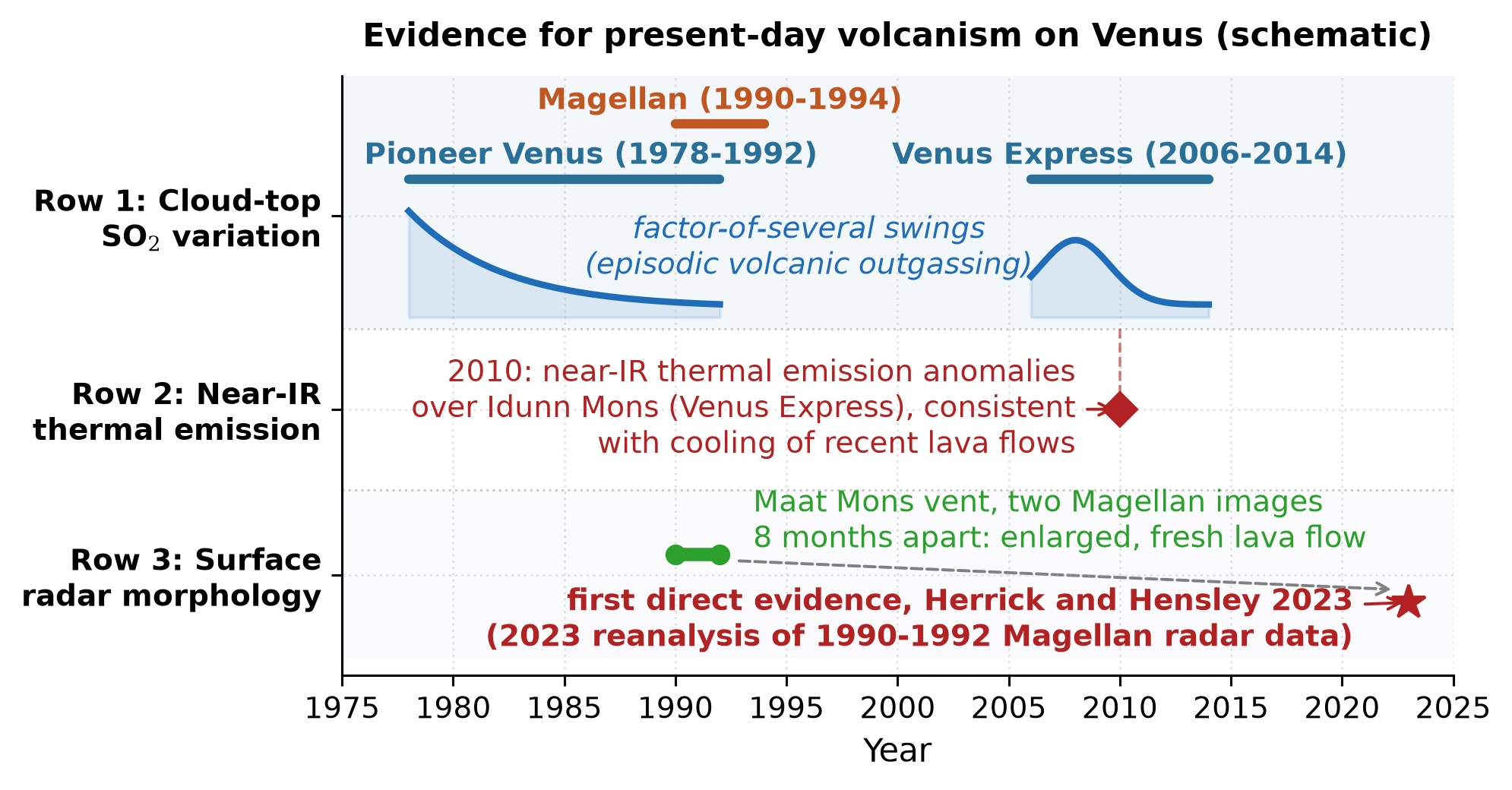
Fig. 9.34 Schematic timeline of the evidence for present-day volcanic activity on Venus. Top row: the coverage of Pioneer Venus (1978 to 1992), Magellan (1990 to 1994) and Venus Express (2006 to 2014), with a qualitative sketch of the factor-of-several swings in cloud-top SO\(_2\) observed during the Pioneer Venus and Venus Express eras (no numerical values implied). Middle row: the Venus Express near-infrared thermal emission anomalies over Idunn Mons, reported in 2010 and consistent with cooling of recent lava flows. Bottom row: the change in a vent on the flank of Maat Mons between two Magellan radar images taken 8 months apart, identified by Herrick and Hensley [2023] as the first direct evidence of an eruption. Course-original figure.#
9.4. Part 3: Comparative payoff#
9.4.1. Why did Earth and Venus diverge?#
Earth and Venus began from similar initial conditions but followed divergent paths driven by four physical inputs and amplifying nonlinear feedbacks.
The first input is solar flux: at \(0.723\) AU, Venus receives \(1.91 \times\) the solar flux of Earth at \(1\) AU. Today, Venus lies above the Simpson-Nakajima limit and Earth sits below it, but under a faint young Sun early Venus was near this threshold, governed by cloud feedbacks. An orbital difference of \(0.05\) AU could have swapped their evolutionary outcomes.
The second input is water delivery: both planets accreted in the same disk region with similar initial water inventories. Mantle isotopic tracers suggest that water, if it arrived with the carbonaceous material, was delivered mainly during main accretion rather than with the late veneer [Dauphas, 2017] (Fig. 9.35).
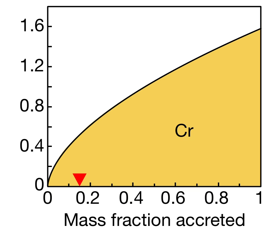
Fig. 9.35 Probability density function for the chromium-bearing fraction of Earth’s accreting mass as a function of the cumulative accreted mass fraction, from Dauphas [2017] (Cr panel of their five-isotope Fig. 1). In the paper’s notation, \(x_{0.95} = 0.85\) for Cr: \(95\%\) of Earth’s present mantle Cr inventory arrived during the final \(85\%\) of accretion, and the red triangle on the \(x\)-axis marks the start of this terminal window at \(1 - x_{0.95} = 0.15\). Mass-proportional delivery would give \(x_{0.95} = 0.95\), so Cr is delivered approximately proportionally to accreted mass (described by the paper as “nearly linear”), in contrast to Mo and Ru, which are strongly back-loaded toward the final stages of accretion. Combined with the O, Ti, Ni, Mo, and Ru tracers from the same study (not reproduced here), Dauphas [2017] reconstruct three accretion stages: stage I (\(0\text{--}60\%\) of Earth’s mass) is best fit by \(\sim 51\%\) enstatite-meteorite-like (E-type) plus \(\sim 40\%\) ordinary-chondrite plus \(\sim 9\%\) carbonaceous-chondrite (CO/CV) material; stages II (\(60\text{--}99.5\%\)) and III (the last \(0.5\%\), the “late veneer”) are essentially \(100\%\) E-type. The carbonaceous component, and therefore the bulk of Earth’s water if it was delivered with that material, was concentrated in the early stages of main accretion rather than in the late veneer.#
Water retention diverged as each planet cooled: Earth condensed an ocean persisting for \(4\) Gyr, whereas on Venus water never condensed or was lost to a runaway greenhouse.
The third input is rotation rate: Venus rotates retrograde with a \(243\)-day period, much slower than Earth’s \(24\)-hour rotation, driving zonal super-rotation instead of mid-latitude cells and altering cloud albedo. Slow rotation may also weaken the organisation of core convection, which may help explain why Venus lacks an intrinsic magnetic field.
The water-loss redox pump connects atmospheric evolution to early water loss (Fig. 9.36). Retaining surface water left Earth with a moderately oxidising mantle and a \(1\)-bar \(\mathrm{N_2}\) atmosphere. On Venus, hydrogen escape oxidised the interior, generating a hot \(\mathrm{CO_2}\)-dominated atmosphere with depleted \(\mathrm{N_2}\) [Wordsworth, 2016].
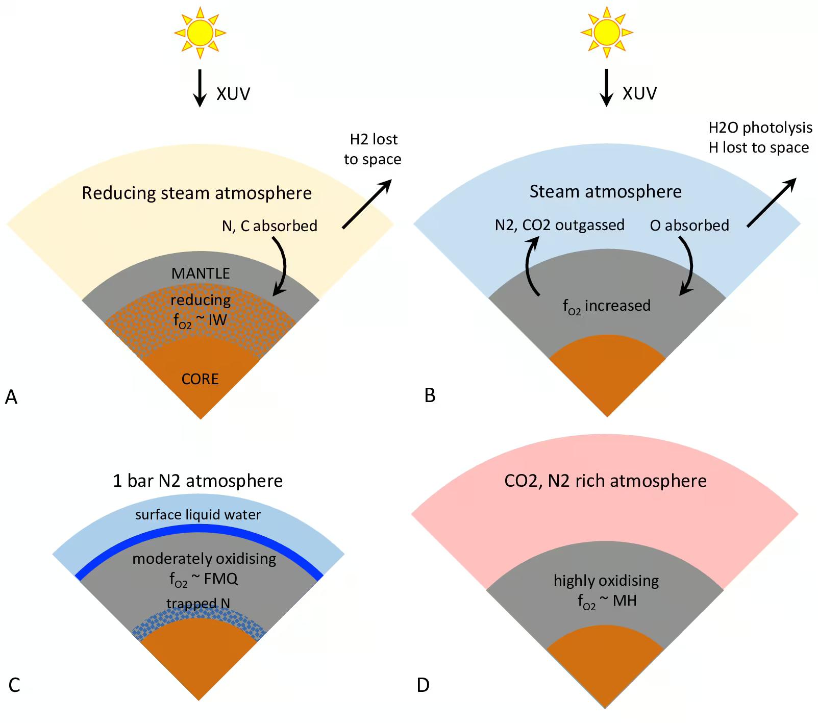
Fig. 9.36 Schematic of the water-loss redox pump linking atmospheric \(\mathrm{N_2}\) inventories to early water-loss histories, from Wordsworth [2016]. Earth evolves to a \(1\)-bar \(\mathrm{N_2}\) atmosphere over a moderately oxidising mantle with liquid water, whereas hydrogen escape on Venus leaves a hot \(\mathrm{CO_2}\)-dominated atmosphere over an oxidised interior.#
The fourth input is tectonic regime: Earth operates in mobile-lid plate tectonics, whereas Venus is in a stagnant-lid regime. Because water weakens mantle olivine and enables subduction, desiccation may have stiffened Venus’ lithosphere and shut down plate tectonics and climate-buffering cycles (Fig. 9.37).
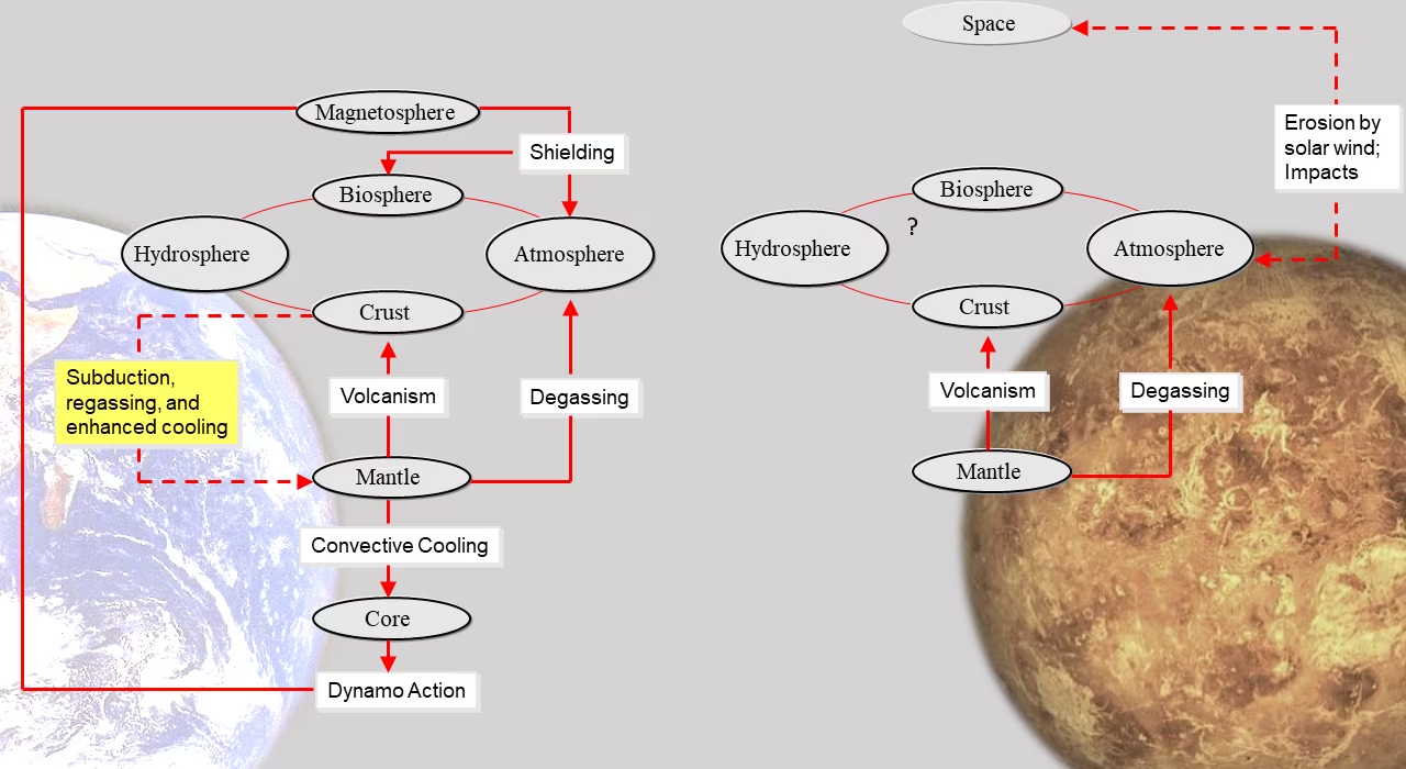
Fig. 9.37 System diagram comparing climate and interior couplings of Earth (left) and Venus (right), from Gillmann et al. [2022]. Earth’s closed system couples mantle convection, plate tectonics, volcanism, fluids, and dynamo, whereas Venus’ open system lacks subduction, surface water, and a magnetic dynamo.#
9.4.2. The carbonate-silicate cycle failure mode on Venus#
The carbonate-silicate cycle is the negative feedback that has stabilised Earth’s climate over \(4\) Gyr (Lecture 6). The cycle requires three essential components: a \(\mathrm{CO_2}\) source (volcanism), a sink (silicate weathering and carbonate burial), and a return leg (subduction). Earth has all three, whereas Venus retains only the source.
When Venus lost its surface liquid water, the silicate weathering sink stopped operating. The reason is that dissolving silicate minerals to precipitate carbonates requires water. Volcanism continued releasing \(\mathrm{CO_2}\) from the interior, and with the source active and the sink shut down, atmospheric \(\mathrm{CO_2}\) accumulated to the present level of \(\sim 92\) bar. In the absence of subduction, Venus also lacks a return leg to recycle crustal carbon back into the mantle. Fig. 9.38 shows this sequence in a coupled interior-atmosphere model: weathering holds the surface temperate for about 0.9 Gyr, then the crustal carbonate decarbonates and the atmospheric reservoir climbs to a Venus-like state.
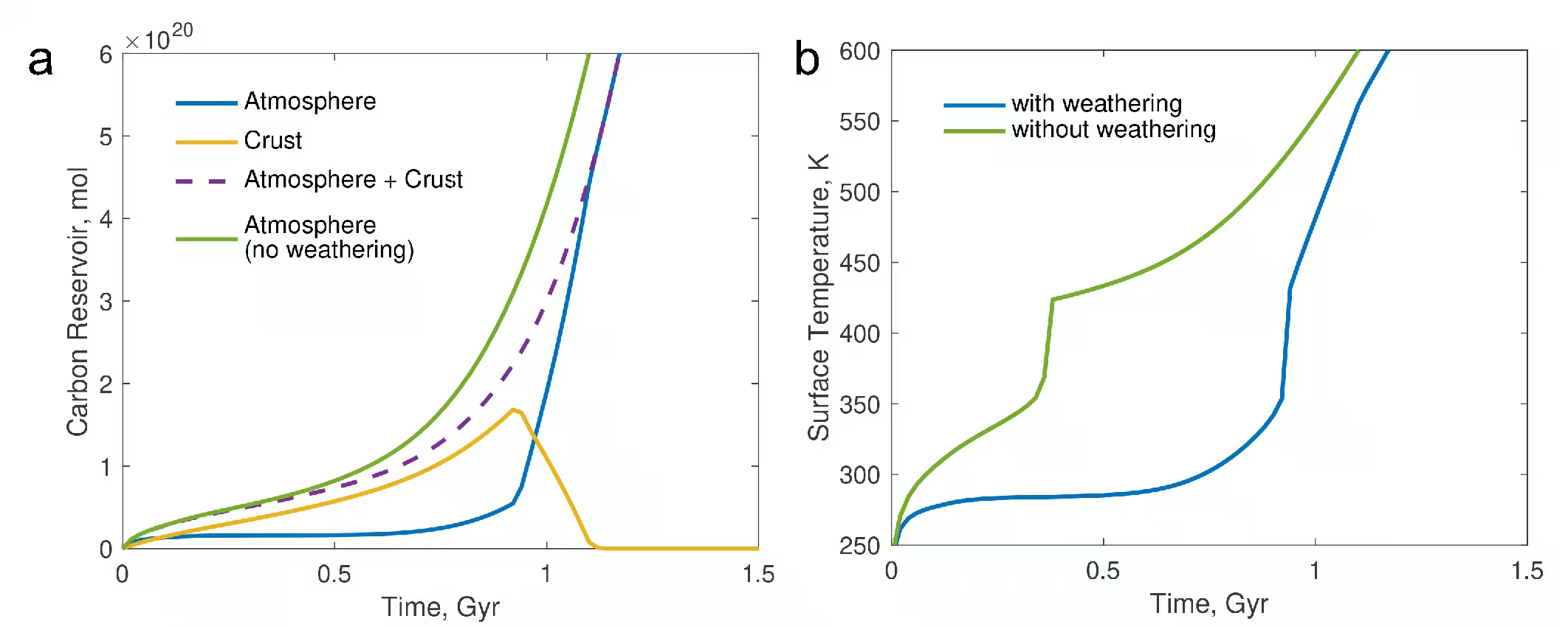
Fig. 9.38 Reference scenario for the coupled interior-atmosphere evolution of a stagnant-lid Venus from panels (a) and (b) of Höning et al. [2021] Fig. 3. Left panel: carbon reservoirs (atmosphere, crust, atmosphere+crust, atmosphere with weathering switched off) as a function of time after solidification. Right panel: surface temperature with (blue) and without (green) silicate weathering. Surface weathering keeps the planet temperate for \(\sim 0.9\) Gyr; once water is lost, decarbonation drives the runaway accumulation of \(\mathrm{CO_2}\) to a Venus-like end state. Reproduced from Höning et al. [2021], Fig. 3a and 3b.#
Earth and Venus acquired similar amounts of carbon during accretion, but the carbon is distributed differently. Earth’s crustal and surface carbon reservoir totals on the order of \(10^{20}\) kg, equivalent to \(\sim 100\) bar of atmospheric \(\mathrm{CO_2}\) [Catling and Kasting, 2017]. Venus holds a comparable inventory of \(92\) bar entirely in its atmosphere. On Earth, almost all carbon is stored in crustal carbonates and the mantle, leaving only a few hundred ppm in the atmosphere. On Venus, cycle failure has left nearly all carbon in the atmosphere.
This cycle failure is irreversible. There is no thermodynamic path back to an Earth-like state because Venus lacks surface oceans, plate tectonics, and geochemical recycling. Once runaway greenhouse conditions push a planet past the inner edge of the habitable zone, it cannot recover. The carbonate-silicate thermostat operates only within bounded conditions, outside of which it breaks irreversibly.
9.4.3. What this means for habitability#
The habitable zone is classically defined as the range of orbital distances where an Earth-like planet can support liquid surface water. However, stellar luminosity increases over time. This shifts the inner edge outward. A planet that enters a runaway greenhouse and loses its water cannot become habitable again later simply because stellar conditions evolve. Habitability is therefore determined by the integrated history of solar flux, water inventory, and feedback systems rather than instantaneous orbital location. The TRAPPIST-1 system in Fig. 9.39 makes the same point for exoplanets: three of its planets sit in the classical habitable zone, yet whether any of them kept its water depends on its history around an M dwarf (Lecture 13).
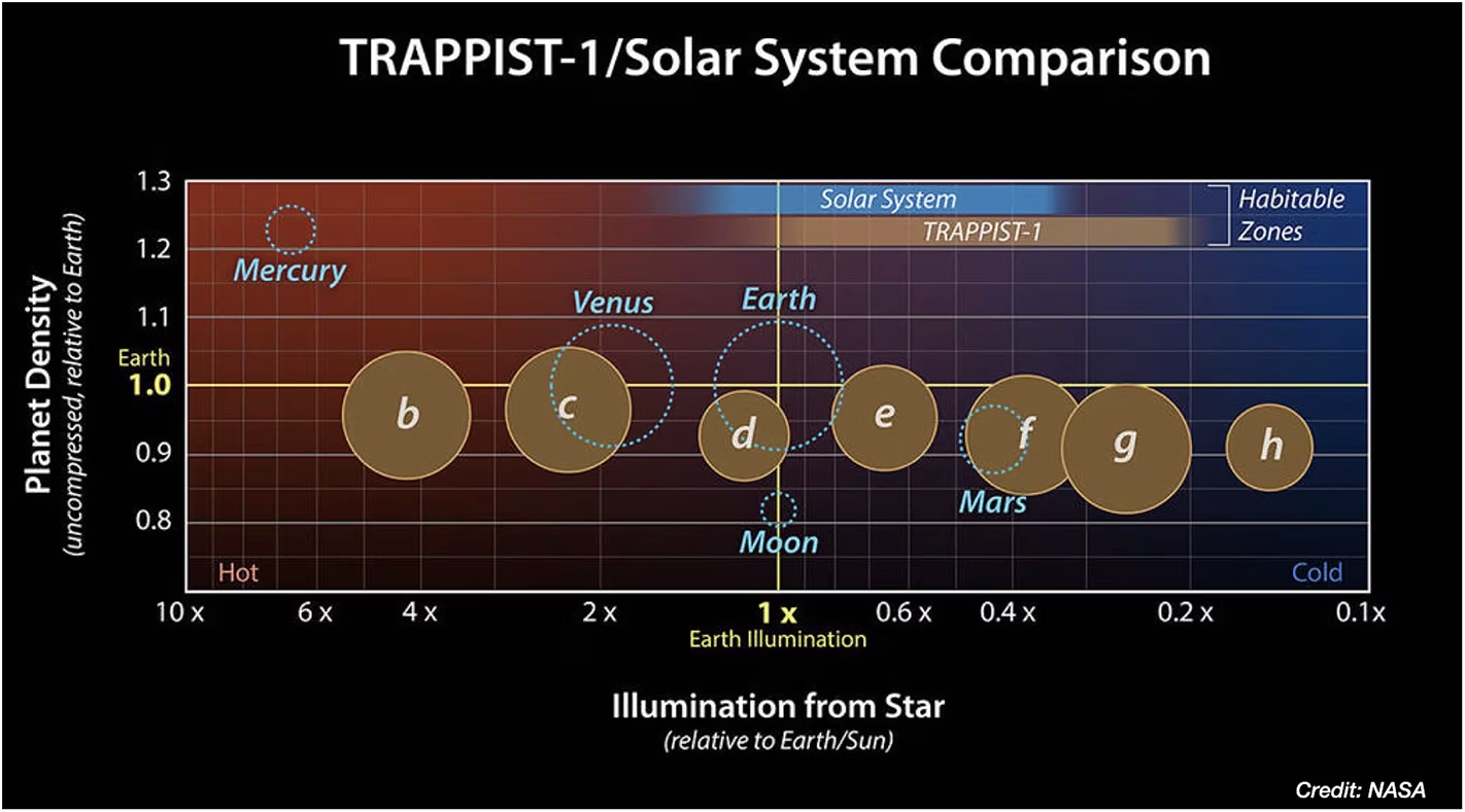
Fig. 9.39 Comparison of the seven TRAPPIST-1 planets (b through h) with the inner Solar System (Mercury, Venus, Earth, Mars), in the plane of planetary density (vertical) versus stellar illumination (horizontal, in units of Earth’s illumination). The blue band marks the classical habitable zone of the Solar System and the tan band that of TRAPPIST-1. Three of the TRAPPIST-1 planets (e, f, g) lie within the habitable zone, and TRAPPIST-1 c receives an illumination similar to Venus. Whether any of these planets actually retain surface water depends on their history (formation, atmospheric evolution, escape) and not just on their current orbital location. Image credit: NASA/JPL-Caltech (PIA22093).#
Earth and Venus exemplify this principle. Earth remains habitable inside the inner edge because the carbonate-silicate thermostat has regulated its climate. Venus sits outside the inner edge today, and either was always outside it or crossed it at some point in the past. The contrast between Earth at \(1\) AU and Venus at \(0.7\) AU is the result of a sensitive balance between radiative input, water inventory, tectonic regime, and biospheric feedback. Applying these lessons to exoplanets requires climate-evolution models that follow a planet through its full history, which is the focus of Lecture 13.
9.4.4. Recent advances and upcoming missions#
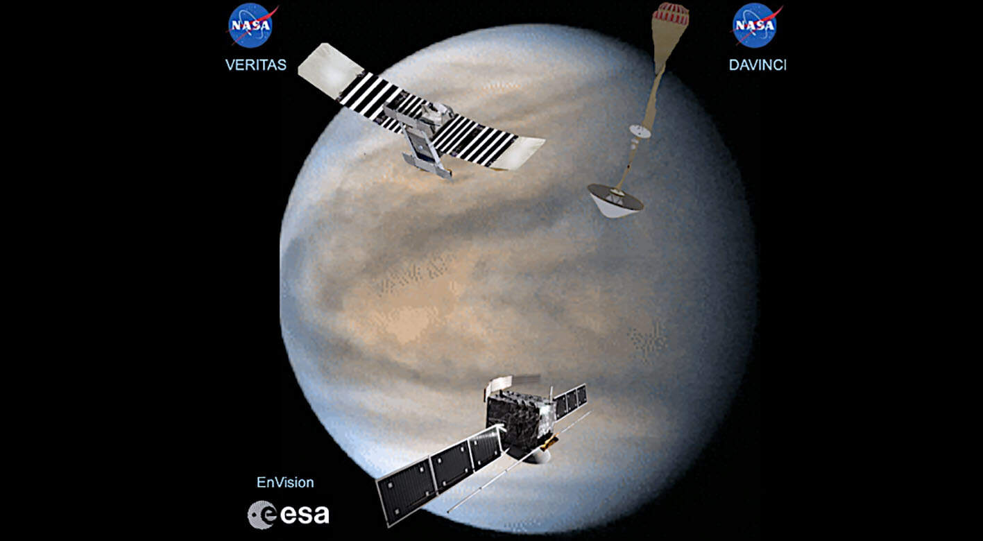
Fig. 9.40 Artist’s rendering of the three Venus missions of the 2030s against a global view of the planet from Akatsuki UV imaging: NASA’s VERITAS (left, top) for radar topography and surface emissivity, NASA’s DAVINCI (right, top) with an atmospheric descent probe, and ESA’s EnVision (below) for radar mapping, atmospheric spectroscopy and subsurface sounding. Reproduced from Widemann et al. [2023].#
The 2030s will see two new orbiters and one in-situ descent probe at Venus (Fig. 9.40). NASA’s DAVINCI is scheduled to launch in \(2029\)–\(2030\) and will send an instrumented probe into the atmosphere to measure noble gas isotopic abundances and atmospheric chemistry. These noble gas measurements record atmospheric escape over time. They distinguish between early-loss and late-loss scenarios for Venus’ water history. NASA’s VERITAS, launching no earlier than \(2031\), will obtain global radar topography and near-infrared surface emissivity to determine tessera composition and constrain mantle convection. ESA’s EnVision is expected to launch in \(2031\), using synthetic-aperture radar to search for active volcanism and characterise tessera regions.
9.5. Summary and takeaways#
Earth and Venus are the closest analogue we have to a controlled experiment in comparative planetology. They started from the same protoplanetary reservoir, accreted to similar masses and densities, and probably acquired comparable inventories of water and carbon. The divergence is due to a small set of physical inputs (solar flux, water history, rotation rate, and tectonic regime) coupled by nonlinear feedbacks that turned modest differences in input into qualitatively different end states.
The central piece of physics is the Simpson-Nakajima runaway greenhouse limit: the maximum thermal flux that a water-saturated atmosphere can radiate to space, set by the saturation vapour pressure curve at the temperature of the IR photosphere. This limit, in the range \(280\) to \(310\) W/m\(^2\), defines the inner edge of the habitable zone and is essentially independent of the surface temperature once the atmosphere is optically thick in the IR. A planet whose absorbed solar flux exceeds the limit cannot host a steady state with liquid surface water: the runaway greenhouse drives the ocean into the upper atmosphere, photolyses the water, and loses the hydrogen to space. Earth, at \(1\) AU, sits below the limit; Venus, at \(0.723\) AU, sits well above it.
The carbonate-silicate cycle has stabilised Earth’s climate within the liquid-water window for \(4\) Gyr, but it cannot operate on present Venus because the cycle requires both liquid surface water (for the weathering sink) and active plate tectonics (for the subduction return leg). Volcanic outgassing continued, and atmospheric \(\mathrm{CO_2}\) accumulated to its present \(92\) bar; Earth’s carbon inventory, mostly stored as carbonate rocks, is comparable in magnitude, so the difference is where the carbon ended up.
The D/H ratio of Venus, enriched by a factor of \(\sim\)150 over the terrestrial value, is the clearest evidence for water loss and implies that Venus lost at least \(100\times\) its present water inventory. Whether the loss happened early (during a perpetual magma ocean phase, the Hamano scenario) or late (after a few-Gyr period of habitability, the Way scenario) remains open, and the answer decides whether early Venus was ever habitable.
Key takeaway: Earth’s long-term habitability rests on a coupled set of feedbacks (carbonate-silicate cycle, plate tectonics, biosphere, dynamo) that all require liquid water and active volcanism; Venus shows what happens when the runaway limit is crossed and these feedbacks stop.
9.6. References#
Catling, David C. and Kasting, James F. 2017. Atmospheric Evolution on Inhabited and Lifeless Worlds. Cambridge University Press, Cambridge. doi:10.1017/9781139020558.
Catling, David C. and Zahnle, Kevin J. 2020. “The Archean atmosphere.” Science Advances, 6(9):eaax1420. doi:10.1126/sciadv.aax1420, https://ui.adsabs.harvard.edu/abs/2020SciA....6.1420C/abstract.
Charnay, Benjamin, Forget, François, Wordsworth, Robin, Leconte, Jérémy, Millour, Ehouarn, Codron, Francis, and Spiga, Aymeric. 2013. “Exploring the faint young Sun problem and the possible climates of the Archean Earth with a 3-D GCM.” Journal of Geophysical Research: Atmospheres, 118(18):10,414–10,431. doi:10.1002/jgrd.50808, arXiv:1310.4286, https://arxiv.org/abs/1310.4286.
Constantinou, Tereza, Shorttle, Oliver, and Rimmer, Paul B. 2024. “A dry Venusian interior constrained by atmospheric chemistry.” Nature Astronomy, 9:189–198. doi:10.1038/s41550-024-02414-5, arXiv:2412.01879, https://arxiv.org/abs/2412.01879.
Dauphas, Nicolas. 2017. “The isotopic nature of the Earth's accreting material through time.” Nature, 541(7638):521–524. doi:10.1038/nature20830, https://ui.adsabs.harvard.edu/abs/2017Natur.541..521D/abstract.
Dodd, Matthew S., Papineau, Dominic, Grenne, Tor, Slack, John F., Rittner, Martin, Pirajno, Franco, O'Neil, Jonathan, and Little, Crispin T. S. 2017. “Evidence for early life in Earth's oldest hydrothermal vent precipitates.” Nature, 543(7643):60–64. doi:10.1038/nature21377, https://ui.adsabs.harvard.edu/abs/2017Natur.543...60D/abstract.
Donahue, T. M., Grinspoon, D. H., Hartle, R. E., and Hodges, R. R. 1997. “Ion/neutral escape of hydrogen and deuterium: evolution of water.” In Bougher, S. W., Hunten, D. M., and Phillips, R. J., editors, Venus II: Geology, Geophysics, Atmosphere, and Solar Wind Environment, pages 385. University of Arizona Press. https://ui.adsabs.harvard.edu/abs/1997veii.conf..385D/abstract.
Donahue, T. M., Hoffman, J. H., Hodges, R. R., and Watson, A. J. 1982. “Venus was wet: a measurement of the ratio of deuterium to hydrogen.” Science, 216(4546):630–633. doi:10.1126/science.216.4546.630, https://ui.adsabs.harvard.edu/abs/1982Sci...216..630D/abstract.
Dziewonski, Adam M. and Anderson, Don L. 1981. “Preliminary reference Earth model.” Physics of the Earth and Planetary Interiors, 25(4):297–356. doi:10.1016/0031-9201(81)90046-7, https://ui.adsabs.harvard.edu/abs/1981PEPI...25..297D/abstract.
Feulner, Georg. 2012. “The faint young Sun problem.” Reviews of Geophysics, 50(2):RG2006. doi:10.1029/2011RG000375, https://ui.adsabs.harvard.edu/abs/2012RvGeo..50.2006F/abstract.
Gibson, Timothy M., Shih, Patrick M., Cumming, Vivien M., Fischer, Woodward W., Crockford, Peter W., Hodgskiss, Malcolm S. W., Wörndle, Sarah, Creaser, Robert A., Rainbird, Robert H., Skulski, Thomas M., and Halverson, Galen P. 2018. “Precise age of Bangiomorpha pubescens dates the origin of eukaryotic photosynthesis.” Geology, 46(2):135–138. doi:10.1130/G39829.1, https://ui.adsabs.harvard.edu/doi/10.1130/G39829.1/abstract.
Gillmann, Cedric, Way, M. J., Avice, Guillaume, Breuer, Doris, Golabek, Gregor J., Höning, Dennis, Krissansen-Totton, Joshua, Lammer, Helmut, O'Rourke, Joseph G., Persson, Moa, Plesa, Ana-Catalina, Salvador, Arnaud, Scherf, Manuel, and Zolotov, Mikhail Yu. 2022. “The long-term evolution of the atmosphere of Venus: processes and feedback mechanisms.” Space Science Reviews, 218(7):56. doi:10.1007/s11214-022-00924-0, https://ui.adsabs.harvard.edu/abs/2022SSRv..218...56G/abstract.
Goldblatt, Colin, Robinson, Tyler D., Zahnle, Kevin J., and Crisp, David. 2013. “Low simulated radiation limit for runaway greenhouse climates.” Nature Geoscience, 6(8):661–667. doi:10.1038/ngeo1892, https://ui.adsabs.harvard.edu/abs/2013NatGe...6..661G/abstract.
Gradstein, Felix M., Ogg, James G., Schmitz, Mark D., and Ogg, Gabi M., editors. 2020. Geologic Time Scale 2020. Elsevier. doi:10.1016/C2020-1-02369-3, https://www.sciencedirect.com/book/9780128243602/geologic-time-scale-2020.
Hamano, Keiko, Abe, Yutaka, and Genda, Hidenori. 2013. “Emergence of two types of terrestrial planet on solidification of magma ocean.” Nature, 497(7451):607–610. doi:10.1038/nature12163, https://ui.adsabs.harvard.edu/abs/2013Natur.497..607H/abstract.
Herrick, Robert R. and Hensley, Scott. 2023. “Surface changes observed on a Venusian volcano during the Magellan mission.” Science, 379(6638):1205–1208. doi:10.1126/science.abm7735, https://ui.adsabs.harvard.edu/abs/2023Sci...379.1205H/abstract.
Hoffman, Paul F., Abbot, Dorian S., Ashkenazy, Yosef, Benn, Douglas I., Brocks, Jochen J., Cohen, Phoebe A., Cox, Grant M., Creveling, Jessica R., Donnadieu, Yannick, Erwin, Douglas H., Fairchild, Ian J., Ferreira, David, Goodman, Jason C., Halverson, Galen P., Jansen, Malte F., Le Hir, Guillaume, Love, Gordon D., Macdonald, Francis A., Maloof, Adam C., Partin, Camille A., Ramstein, Gilles, Rose, Brian E. J., Rose, Catherine V., Sadler, Peter M., Tziperman, Eli, Voigt, Aiko, and Warren, Stephen G. 2017. “Snowball Earth climate dynamics and Cryogenian geology–geobiology.” Science Advances, 3(11):e1600983. doi:10.1126/sciadv.1600983, https://ui.adsabs.harvard.edu/abs/2017SciA....3E0983H/abstract.
Hunten, Donald M., Pepin, Robert O., and Walker, James C. G. 1987. “Mass fractionation in hydrodynamic escape.” Icarus, 69(3):532–549. doi:10.1016/0019-1035(87)90022-4, https://ui.adsabs.harvard.edu/abs/1987Icar...69..532H/abstract.
Höning, Dennis, Baumeister, Philipp, Grenfell, John Lee, Tosi, Nicola, and Way, Michael J. 2021. “Early habitability and crustal decarbonation of a stagnant-lid venus.” Journal of Geophysical Research: Planets, 126(10):e2021JE006895. doi:10.1029/2021JE006895, arXiv:2109.08756, https://ui.adsabs.harvard.edu/abs/2021JGRE..12606895H/abstract.
Ivanov, Mikhail A. and Head, James W. 2015. “The history of tectonism on Venus: a stratigraphic analysis.” Planetary and Space Science, 113:10–32. doi:10.1016/j.pss.2015.03.016, https://ui.adsabs.harvard.edu/abs/2015P%26SS..113...10I/abstract.
Javaux, Emmanuelle J. and Lepot, Kevin. 2018. “The Paleoproterozoic fossil record: implications for the evolution of the biosphere during Earth's middle-age.” Earth-Science Reviews, 176:68–86. doi:10.1016/j.earscirev.2017.10.001, https://insu.hal.science/insu-03190875v1/document.
Kasting, James F. 1988. “Runaway and moist greenhouse atmospheres and the evolution of Earth and Venus.” Icarus, 74(3):472–494. doi:10.1016/0019-1035(88)90116-9, https://ui.adsabs.harvard.edu/abs/1988Icar...74..472K/abstract.
Kasting, James F., Whitmire, Daniel P., and Reynolds, Ray T. 1993. “Habitable zones around main sequence stars.” Icarus, 101(1):108–128. doi:10.1006/icar.1993.1010, https://ui.adsabs.harvard.edu/abs/1993Icar..101..108K/abstract.
Kopparapu, Ravi Kumar, Ramirez, Ramses, Kasting, James F., Eymet, Vincent, Robinson, Tyler D., Mahadevan, Suvrath, Terrien, Ryan C., Domagal-Goldman, Shawn, Meadows, Victoria, and Deshpande, Rohit. 2013. “Habitable zones around main-sequence stars: new estimates.” The Astrophysical Journal, 765(2):131. doi:10.1088/0004-637X/765/2/131, arXiv:1301.6674, https://ui.adsabs.harvard.edu/abs/2013ApJ...765..131K/abstract.
Krissansen-Totton, Joshua, Arney, Giada N., and Catling, David C. 2018. “Constraining the climate and ocean pH of the early Earth with a geological carbon cycle model.” Proceedings of the National Academy of Sciences, 115(16):4105–4110. doi:10.1073/pnas.1721296115, arXiv:1804.00219, https://ui.adsabs.harvard.edu/abs/2018PNAS..115.4105K/abstract.
Lammer, Helmut, Zerkle, Aubrey L., Gebauer, Stefanie, Tosi, Nicola, Noack, Lena, Scherf, Manuel, Pilat-Lohinger, Elke, Gudel, Manuel, Grenfell, John Lee, Godolt, Mareike, and Nikolaou, Athanasia. 2018. “Origin and evolution of the atmospheres of early Venus, Earth and Mars.” Astronomy and Astrophysics Review, 26(1):2. doi:10.1007/s00159-018-0108-y, https://ui.adsabs.harvard.edu/abs/2018A%26ARv..26....2L/abstract.
Lebrun, T., Massol, H., Chassefière, E., Davaille, A., Marcq, E., Sarda, P., Leblanc, F., and Brandeis, G. 2013. “Thermal evolution of an early magma ocean in interaction with the atmosphere.” Journal of Geophysical Research: Planets, 118(6):1155–1176. doi:10.1002/jgre.20068, https://ui.adsabs.harvard.edu/abs/2013JGRE..118.1155L/abstract.
Lyons, Timothy W., Reinhard, Christopher T., and Planavsky, Noah J. 2014. “The rise of oxygen in Earth's early ocean and atmosphere.” Nature, 506(7488):307–315. doi:10.1038/nature13068, https://ui.adsabs.harvard.edu/abs/2014Natur.506..307L/abstract.
Mojzsis, S. J., Arrhenius, G., McKeegan, K. D., Harrison, T. M., Nutman, A. P., and Friend, C. R. L. 1996. “Evidence for life on Earth before 3,800 million years ago.” Nature, 384(6604):55–59. doi:10.1038/384055a0, https://ui.adsabs.harvard.edu/abs/1996Natur.384...55M/abstract.
Nakajima, Sho, Hayashi, Yoshi-Yuki, and Abe, Yutaka. 1992. “A study on the runaway greenhouse effect with a one-dimensional radiative-convective equilibrium model.” Journal of the Atmospheric Sciences, 49(23):2256–2266. doi:10.1175/1520-0469(1992)049<2256:ASOTRG>2.0.CO;2, https://ui.adsabs.harvard.edu/abs/1992JAtS...49.2256N/abstract.
Nutman, Allen P., Bennett, Vickie C., Friend, Clark R. L., Van Kranendonk, Martin J., and Chivas, Allan R. 2016. “Rapid emergence of life shown by discovery of 3,700-million-year-old microbial structures.” Nature, 537(7621):535–538. doi:10.1038/nature19355, https://ui.adsabs.harvard.edu/abs/2016Natur.537..535N/abstract.
Schmidt, Gavin A., Ruedy, Reto A., Miller, Ron L., and Lacis, Andy A. 2010. “Attribution of the present-day total greenhouse effect.” Journal of Geophysical Research: Atmospheres. doi:10.1029/2010JD014287, https://ui.adsabs.harvard.edu/doi/10.1029/2010JD014287/abstract.
Seiff, A., Schofield, J. T., Kliore, A. J., Taylor, F. W., Limaye, S. S., Revercomb, H. E., Sromovsky, L. A., Kerzhanovich, V. V., Moroz, V. I., and Marov, M. Ya. 1985. “Models of the structure of the atmosphere of Venus from the surface to 100 kilometers altitude.” Advances in Space Research, 5(11):3–58. doi:10.1016/0273-1177(85)90197-8, https://ui.adsabs.harvard.edu/abs/1985AdSpR...5...3S/abstract.
Smrekar, Suzanne E., Davaille, Anne, and Sotin, Christophe. 2018. “Venus interior structure and dynamics.” Space Science Reviews, 214(5):88. doi:10.1007/s11214-018-0518-1, https://ui.adsabs.harvard.edu/abs/2018SSRv..214...88S/abstract.
Tarduno, John A., Cottrell, Rory D., Watkeys, Michael K., Hofmann, Axel, Doubrovine, Pavel V., Mamajek, Eric E., Liu, Dunji, Sibeck, David G., Neukirch, Levi P., and Usui, Yoichi. 2010. “Geodynamo, solar wind, and magnetopause 3.4 to 3.45 billion years ago.” Science, 327(5970):1238–1240. doi:10.1126/science.1183445, https://ui.adsabs.harvard.edu/abs/2010Sci...327.1238T/abstract.
Tellmann, Silvia, Pätzold, Martin, Häusler, Bernd, Bird, Michael K., and Tyler, G. Leonard. 2009. “Structure of the Venus neutral atmosphere as observed by the radio science experiment VeRa on Venus Express.” Journal of Geophysical Research: Planets, 114(E9):E00B36. doi:10.1029/2008JE003204, https://ui.adsabs.harvard.edu/abs/2009JGRE..114.0B36T/abstract.
Turbet, Martin, Bolmont, Emeline, Chaverot, Guillaume, Ehrenreich, David, Leconte, Jérémy, and Marcq, Emmanuel. 2021. “Day–night cloud asymmetry prevents early oceans on Venus but not on Earth.” Nature, 598(7880):276–280. doi:10.1038/s41586-021-03873-w, https://ui.adsabs.harvard.edu/abs/2021Natur.598..276T/abstract.
Walker, James C. G., Hays, P. B., and Kasting, James F. 1981. “A negative feedback mechanism for the long-term stabilization of Earth's surface temperature.” Journal of Geophysical Research: Oceans, 86(C10):9776–9782. doi:10.1029/JC086iC10p09776, https://ui.adsabs.harvard.edu/abs/1981JGR....86.9776W/abstract.
Way, Michael J., Del Genio, Anthony D., Kiang, Nancy Y., Sohl, Linda E., Grinspoon, David H., Aleinov, Igor, Kelley, Maxwell, and Clune, Thomas. 2016. “Was Venus the first habitable world of our solar system?.” Geophysical Research Letters, 43(16):8376–8383. doi:10.1002/2016GL069790, https://ui.adsabs.harvard.edu/abs/2016GeoRL..43.8376W/abstract.
Widemann, Thomas, Smrekar, Suzanne E., Garvin, James B., Straume-Lindner, Ann Carine, Ocampo, Adriana C., Schulte, Mitchell D., Voirin, Thomas, Hensley, Scott, Dyar, M. Darby, Whitten, Jennifer L., Nunes, Daniel C., Getty, Stephanie A., Arney, Giada N., Johnson, Natasha M., Kohler, Erika, Spohn, Tilman, O'Rourke, Joseph G., Wilson, Colin F., Way, Michael J., Ostberg, Colby, Westall, Frances, Höning, Dennis, Bauer, Seth, Bruzzone, Lorenzo, Cascioli, Gael, Dumoulin, Caroline, Marcq, Emmanuel, Mazarico, Erwan, Nakajima, Miki, Plesa, Ana-Catalina, Quick, Lynnae C., Salvador, Arnaud, Solomatov, Viktor, Sori, Michael M., Sundqvist, Hans, Withers, Paul, Boukrouche, Ryan, Eggl, Siegfried, Glaze, Lori S., Helbert, Jörn, Iess, Luciano, Korablev, Oleg, Lefevre, Maxence, Lognonné, Philippe, and Muñoz, Antonio García. 2023. “Venus evolution through time: key science questions, selected mission concepts and future investigations.” Space Science Reviews, 219(7):56. doi:10.1007/s11214-023-00992-w, https://ui.adsabs.harvard.edu/abs/2023SSRv..219...56W/abstract.
Wilde, Simon A., Valley, John W., Peck, William H., and Graham, Colin M. 2001. “Evidence from detrital zircons for the existence of continental crust and oceans on the Earth 4.4 Gyr ago.” Nature, 409(6817):175–178. doi:10.1038/35051550, https://ui.adsabs.harvard.edu/abs/2001Natur.409..175W/abstract.
Wordsworth, R. D. 2016. “Atmospheric nitrogen evolution on Earth and Venus.” Earth and Planetary Science Letters, 447:103–111. doi:10.1016/j.epsl.2016.04.002, arXiv:1605.07718, https://arxiv.org/abs/1605.07718.
Wordsworth, R. D. and Pierrehumbert, R. T. 2013. “Water loss from terrestrial planets with CO₂-rich atmospheres.” The Astrophysical Journal, 778(2):154. doi:10.1088/0004-637X/778/2/154, arXiv:1306.3266, https://ui.adsabs.harvard.edu/abs/2013ApJ...778..154W/abstract.
Wordsworth, R. D. and Pierrehumbert, R. T. 2014. “Abiotic oxygen-dominated atmospheres on terrestrial habitable zone planets.” The Astrophysical Journal Letters, 785(2):L20. doi:10.1088/2041-8205/785/2/L20, arXiv:1403.2713, https://ui.adsabs.harvard.edu/abs/2014ApJ...785L..20W/abstract.
Zahnle, Kevin, Arndt, Nick, Cockell, Charles, Halliday, Alex, Nisbet, Euan, Selsis, Franck, and Sleep, Norman H. 2007. “Emergence of a habitable planet.” Space Science Reviews, 129(1–3):35–78. doi:10.1007/s11214-007-9225-z, https://ui.adsabs.harvard.edu/abs/2007SSRv..129...35Z/abstract.
NASA Jet Propulsion Laboratory. 2026. Planetary physical parameters. NASA Solar System Dynamics, Caltech/JPL. Values derive from the IAU/IAG Working Group report (Archinal et al. 2018, Celestial Mechanics and Dynamical Astronomy 130:22) and current GM estimates. https://ssd.jpl.nasa.gov/planets/phys_par.html.
NASA Jet Propulsion Laboratory. 2026. Planetary physical parameters: Venus. NASA Solar System Dynamics, Caltech/JPL. Values derive from the IAU/IAG Working Group report (Archinal et al. 2018, Celestial Mechanics and Dynamical Astronomy 130:22) and current GM estimates. https://ssd.jpl.nasa.gov/planets/phys_par.html.